
新NISA、一括投資か分割投資か?S&P 500データでのシミュレーション

新NISAも始まりオルカン、S&P500などの投資信託やETFに人気が集まっています。投資手法もいろいろありますが一括投資が良いのか、分割投資が良いのか、という記事は多く見かけます。ドルコスト平均法が良い、という記事も多いのですが本当にそうでしょうか?あるいは一括投資が理論的に優れるという記事もあります。実際にS&P500のデータを用いてシミュレーションしてみます。
まずinvesting.comから過去のS&P500データをダウンロードします。2011年から2023年までの13年間を抽出したのが下記のデータになります。
このデータを用いて実際にPythonでシミュレーションしてみます。今回はJupyter Notebookを用いています。
import pandas as pd
import numpy as np
from datetime import datetime
from matplotlib import pyplot as plt
from pandas.plotting import register_matplotlib_converters

register_matplotlib_converters()

# データの読み込み
df = pd.read_csv('data2023.csv')
df['date'] = pd.to_datetime(df['date'])
df.set_index('date', inplace=True)

# null値のある行を削除
df = df.dropna(subset=['value'])

# 解析の開始期間と終了期間を設定
start_date = "1995-01-01"  # 開始日を設定
end_date = "2025-01-01"    # 終了日を設定

# 指定した期間のデータだけを保持
df = df[(df.index >= start_date) & (df.index <= end_date)]

# 投資戦略の設定(月次投資と一括投資を含む)
strategies = ["monthly_investment", "lump_sum_investment"]
strategy_labels = ["Monthly Investment", "Lump Sum Investment"]

# 各戦略についてシミュレーションを行う
for strategy in strategies:
    total_investment = 0
    total_shares = 0
    cash = 100000
    df[strategy + '_shares'] = 0
    df[strategy + '_investment'] = 0
    df[strategy + '_profit'] = 0
    df[strategy + '_cash'] = cash

    for i, row in df.iterrows():
        month = i.month
        next_month = df.index[df.index > i].month[0] if df.index[df.index > i].month.size > 0 else month
        is_last_row = i == df.index[-1]

        if strategy == "monthly_investment" and (i == df.index[0] or month != df.index[df.index < i][-1].month) and not is_last_row:
            investment = cash
        elif strategy == "lump_sum_investment" and i == df.index[0]:  # Lump sum investment at the first day
            investment = 100000 * len(df.resample('M'))  # Monthly investment multiplied by number of months
        else:
            investment = 0

        shares = investment // row['value']
        cost = shares * row['value']
        cash = cash - cost + (100000 if month != next_month else 0)

        total_investment += cost
        total_shares += shares

        df.at[i, strategy + '_shares'] = total_shares
        df.at[i, strategy + '_investment'] = total_investment
        df.at[i, strategy + '_profit'] = total_shares * row['value'] - total_investment
        df.at[i, strategy + '_cash'] = cash

# 利益をプロット
fig, ax1 = plt.subplots(figsize=(20, 10))

# 利益のプロット
for strategy, label in zip(strategies, strategy_labels):
    ax1.plot(df.index, df[strategy + '_profit'], label=label)
ax1.set_xlabel('Date')
ax1.set_ylabel('Profit in $')
ax1.legend()
ax1.grid(True)

plt.show()

# 株価のプロット
ax2 = ax1.twinx()  # instantiate a second axes that shares the same x-axis
ax2.plot(df.index, df['value'], label='Stock Price', color='gray', linestyle='dashed')
ax2.set_ylabel('Stock Price in $')  # we already handled the x-label with ax1

# Adjust the scale of the stock price
ax2.set_ylim([df['value'].min() - 50, df['value'].max() + 50])

# Combining legends from both the axis
lines1, labels1 = ax1.get_legend_handles_labels()
lines2, labels2 = ax2.get_legend_handles_labels()
ax2.legend(lines1 + lines2, labels1 + labels2, loc='upper left')

fig.tight_layout()  # otherwise the right y-label is slightly clipped

plt.show()

# 投資額のプロット
fig, ax3 = plt.subplots(figsize=(20, 10))  # define a new figure and axis for investment
for strategy, label in zip(strategies, strategy_labels):
    ax3.plot(df.index, df[strategy + '_investment'], label=label)  # use ax3 instead of axs[1]
ax3.set_xlabel('Date')
ax3.set_ylabel('Investment in $')
ax3.legend()
ax3.grid(True)

plt.show()

# 株価のみのプロット
fig, ax = plt.subplots(figsize=(20, 10))
ax.plot(df.index, df['value'], color='blue', label='Stock Price')
ax.set_xlabel('Date')
ax.set_ylabel('Stock Price in $')
ax.legend()
ax.grid(True)
plt.show()

# 最終結果の表示
for strategy, label in zip(strategies, strategy_labels):
    final_profit = df[strategy + '_profit'][-1]
    total_investment = df[strategy + '_investment'][-1]
    final_cash = df[strategy + '_cash'][-1]
    print(f'Final profit for {label}: ${final_profit:.2f}')
    print(f'Total investment for {label}: ${total_investment:.2f}')
    print(f'Final cash for {label}: ${final_cash:.2f}')
    print(f'Return on Investment for {label}: {final_profit/total_investment*100:.2f}%')

# 結果をエクセルファイルに保存
df.to_excel('investment_results.xlsx')
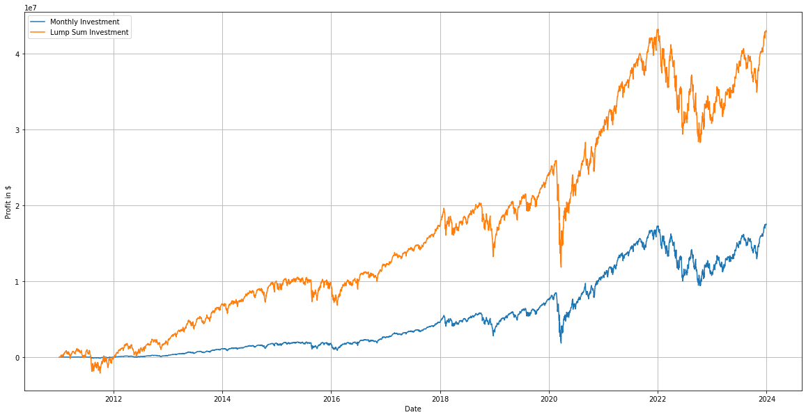
このコードで比較しているのは1)一括投資(最初に全金額を投資)Lump Sum Investment、2)分割投資(月々決まった額を投資)Montyly Investmentの2手法です。実際にコードを出力すると3つのグラフが出力されます。
最初のグラフがパフォーマンスの比較です。
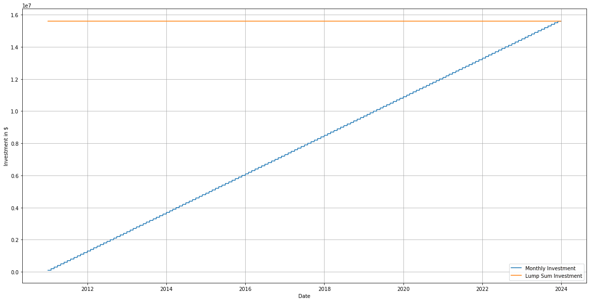
次が総投資額のグラフ、これは両手法で投資額が同じか確認しています。
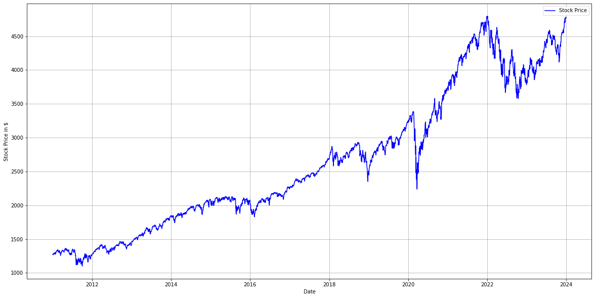
最後が株価のシミュレーションです。
最後に投資結果が出力されます。
Final profit for Monthly Investment: $17466026.00 Total investment for Monthly Investment: $15598434.00 Final cash for Monthly Investment: $1565.00 Return on Investment for Monthly Investment: 111.97% Final profit for Lump Sum Investment: $42902479.00 Total investment for Lump Sum Investment: $15599485.00 Final cash for Lump Sum Investment: $514.00 Return on Investment for Lump Sum Investment: 275.02%
一括投資では275%のリターン(利益)が得られるのに対し分割投資では112%のリターンとなります。
単年度ではどうか
上記のシミュレーションでは13年間の経過で一括投資と分割投資を比較しましたが単年度ではどうでしょうか?新NISAでは1年毎に投資枠が決められています(成長枠投資は120万円/年)。よって1年毎に比較するほうが実際の投資手法の比較としては有効と思います。
先程のコードで下記の部分を変更すると例えば2023年度単年での一括投資と分割投資を比較できます。
# 解析の開始期間と終了期間を設定
start_date = "1995-01-01"  # 開始日を設定
end_date = "2025-01-01"    # 終了日を設定
2023年単年度での比較:一括投資vs分割投資
上記コードを下記に変更して実行します。
# 解析の開始期間と終了期間を設定
start_date = "2023-01-01"  # 開始日を設定
end_date = "2023-12-31"    # 終了日を設定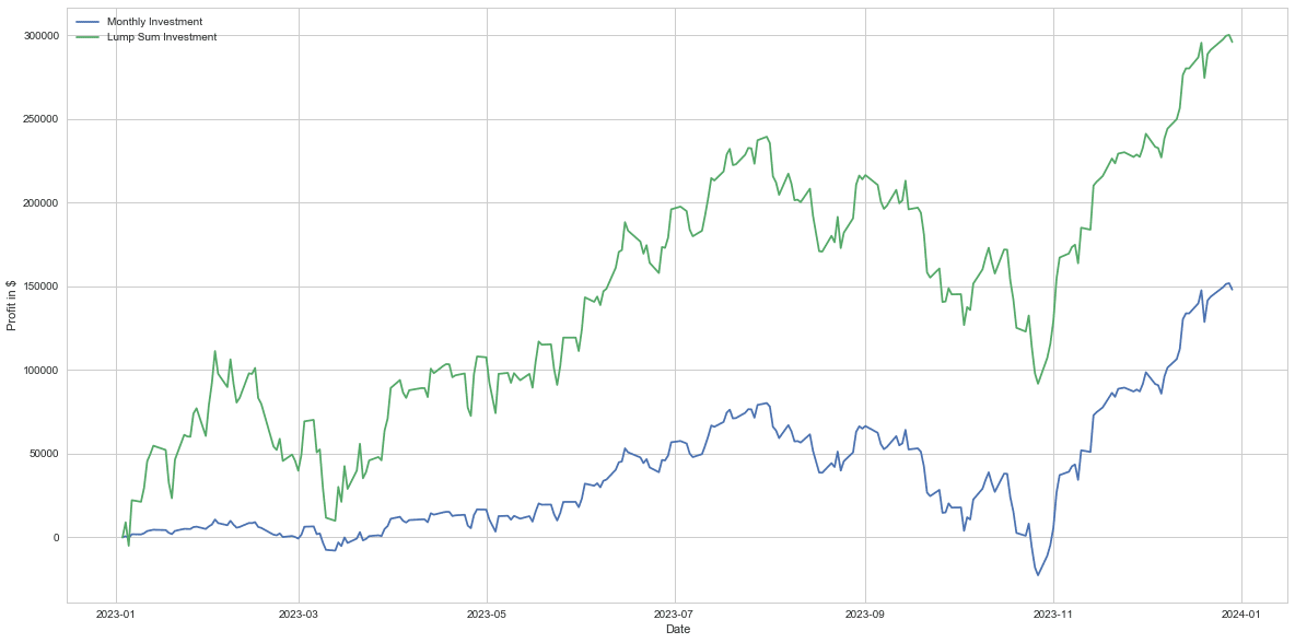
最終的なリターンは
Final profit for Monthly Investment: $148058.00 Total investment for Monthly Investment: $1197033.00 Final cash for Monthly Investment: $2966.00 Return on Investment for Monthly Investment: 12.37% Final profit for Lump Sum Investment: $296000.00 Total investment for Lump Sum Investment: $1196955.00 Final cash for Lump Sum Investment: $3044.00 Return on Investment for Lump Sum Investment: 24.73%
一括投資では24.7%のリターン(利益)が得られるのに対し分割投資では12.4%のリターンとなります。2023年度の株価を見てみますと
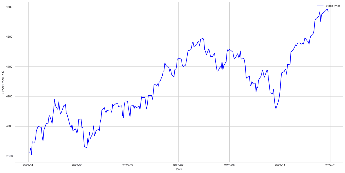
となっております。このような上げ相場では一括投資が分割投資に勝ることは容易にわかります。
2022年度の比較:一括投資vs分割投資
同じように2022年度も比較してみます。
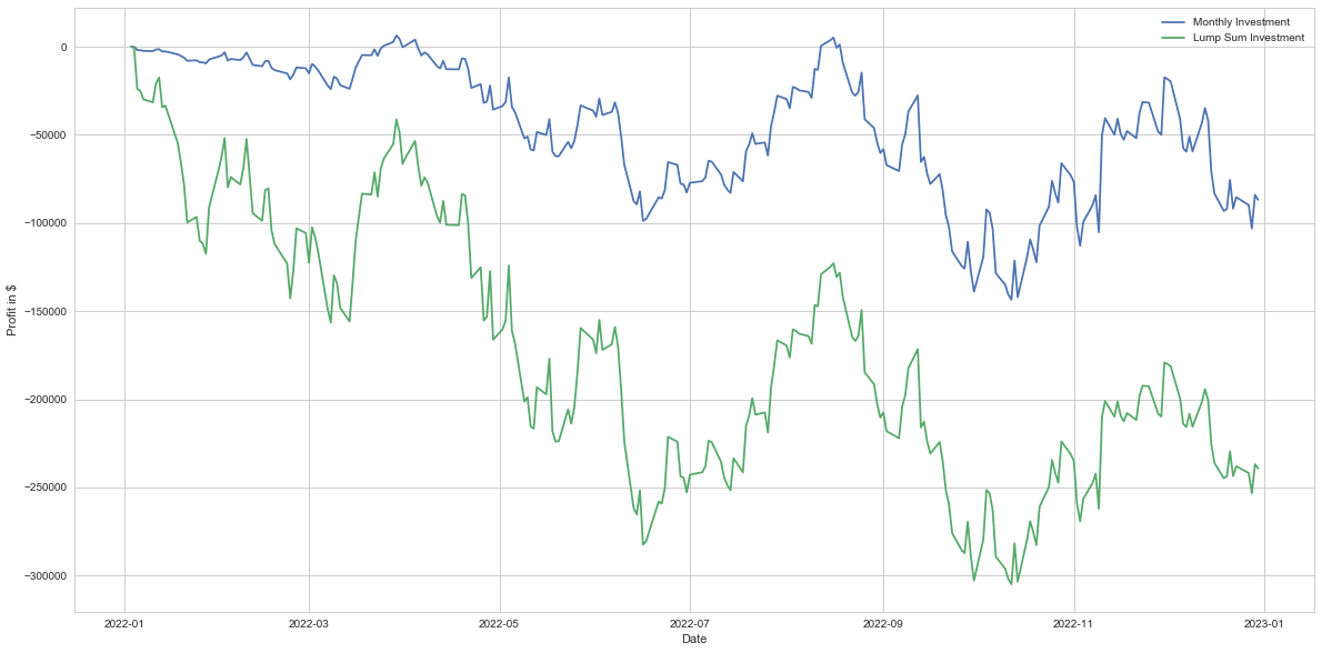
2022年度の投資結果は
Final profit for Monthly Investment: $-86866.00 Total investment for Monthly Investment: $1196482.00 Final cash for Monthly Investment: $3517.00 Return on Investment for Monthly Investment: -7.26% Final profit for Lump Sum Investment: $-239265.00 Total investment for Lump Sum Investment: $1199140.00 Final cash for Lump Sum Investment: $860.00 Return on Investment for Lump Sum Investment: -19.95%
一括投資では-19.95%のロス(損益)が得られるのに対し分割投資では-7.26%のロスに留まります。
2022年度の株価を見てみますと
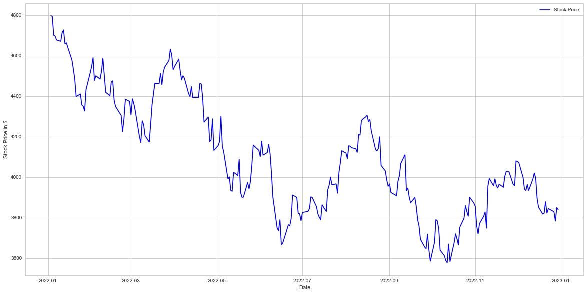
完全な下げ相場であったことがわかります。このように下げ相場の場合は一括投資は大きな損益に繋がります。
2011年から2023年まで13年間での比較(単年毎)
では2011年から2023年の13年間、毎年取引初日に1年分の投資をする一括投資と毎月にわけて購入する分割投資、どちらが優れたパフォーマンスを発揮しているのでしょうか?比較するために新しくコードを書きます。
import pandas as pd

# データの読み込み
df = pd.read_csv('data2023.csv')
df['date'] = pd.to_datetime(df['date'])
df.set_index('date', inplace=True)

# null値のある行を削除
df = df.dropna(subset=['value'])

# データの最初の数行を表示して内容を確認
df.head()

def simulate_investment(df, start_date, end_date, cash=100000):
    """
    特定の期間における投資戦略のシミュレーションを行う関数。

    Args:
    df (DataFrame): 株価データを含むDataFrame。
    start_date (datetime): シミュレーションの開始日。
    end_date (datetime): シミュレーションの終了日。
    cash (int, optional): 初期投資額。デフォルトは100,000。

    Returns:
    dict: 各戦略における最終利益、総投資額、最終現金残高、ROIの辞書。
    """
    # 指定した期間のデータを抽出
    period_df = df[(df.index >= start_date) & (df.index <= end_date)]

    # 投資戦略の設定
    strategies = ["monthly_investment", "lump_sum_investment"]
    results = {}

    for strategy in strategies:
        total_investment = 0
        total_shares = 0
        current_cash = cash

        for i, row in period_df.iterrows():
            month = i.month
            next_month = period_df.index[period_df.index > i].month[0] if period_df.index[period_df.index > i].month.size > 0 else month
            is_last_row = i == period_df.index[-1]

            if strategy == "monthly_investment" and (i == period_df.index[0] or month != period_df.index[period_df.index < i][-1].month) and not is_last_row:
                investment = current_cash
            elif strategy == "lump_sum_investment" and i == period_df.index[0]:
                investment = cash * len(period_df.resample('M'))
            else:
                investment = 0

            shares = investment // row['value']
            cost = shares * row['value']
            current_cash = current_cash - cost + (100000 if month != next_month else 0)

            total_investment += cost
            total_shares += shares

        final_profit = total_shares * period_df['value'][-1] - total_investment
        roi = (final_profit / total_investment) * 100 if total_investment > 0 else 0

        results[strategy] = {
            "final_profit": final_profit,
            "total_investment": total_investment,
            "final_cash": current_cash,
            "roi": roi
        }

    return results

# 2011年から2023年までのシミュレーションを実行
all_years_results = {}

for year in range(2011, 2024):
    start_date = pd.to_datetime(f"{year}-01-01")
    end_date = pd.to_datetime(f"{year}-12-31")
    all_years_results[year] = simulate_investment(df, start_date, end_date)

# 結果を表に変換
all_years_df = pd.DataFrame()

for year, results in all_years_results.items():
    for strategy, metrics in results.items():
        strategy_label = "Monthly Investment" if strategy == "monthly_investment" else "Lump Sum Investment"
        all_years_df = all_years_df.append({
            "Year": year,
            "Strategy": strategy_label,
            "Final Profit": metrics["final_profit"],
            "Total Investment": metrics["total_investment"],
            "Final Cash": metrics["final_cash"],
            "ROI": metrics["roi"]
        }, ignore_index=True)

# 結果を整理
all_years_df_sorted = all_years_df.sort_values(by=["Year", "Strategy"]).reset_index(drop=True)
all_years_df_sorted  # 全ての結果をテーブル形式で表示
実行しますと下記テーブルが出力されます。
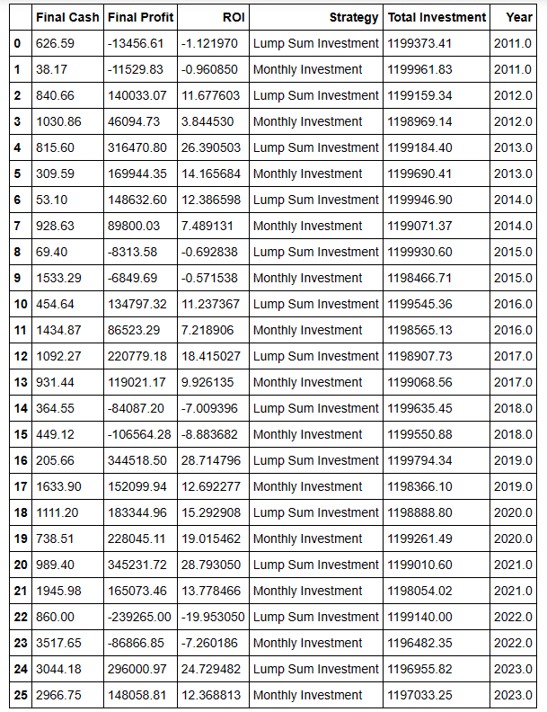
少しわかりにくいですが一括投資の9勝4敗となります。また平均でのROI(投資利益率)は一括投資が11.45%に対して分割投資では6.37%となります。
テーブルをグラフにしてみます。
import matplotlib.pyplot as plt
import seaborn as sns

# グラフのスタイルを設定
sns.set(style="whitegrid")

# 年度ごとに戦略別のROIをプロットする棒グラフ
plt.figure(figsize=(15, 8))
sns.barplot(x="Year", y="ROI", hue="Strategy", data=all_years_df_sorted)

# タイトルとラベルの設定
plt.title('Yearly ROI Comparison between Investment Strategies')
plt.xlabel('Year')
plt.ylabel('ROI (%)')

# 凡例の表示
plt.legend(title='Strategy')

# グラフの表示
plt.show()
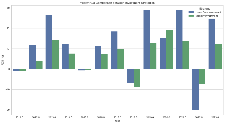
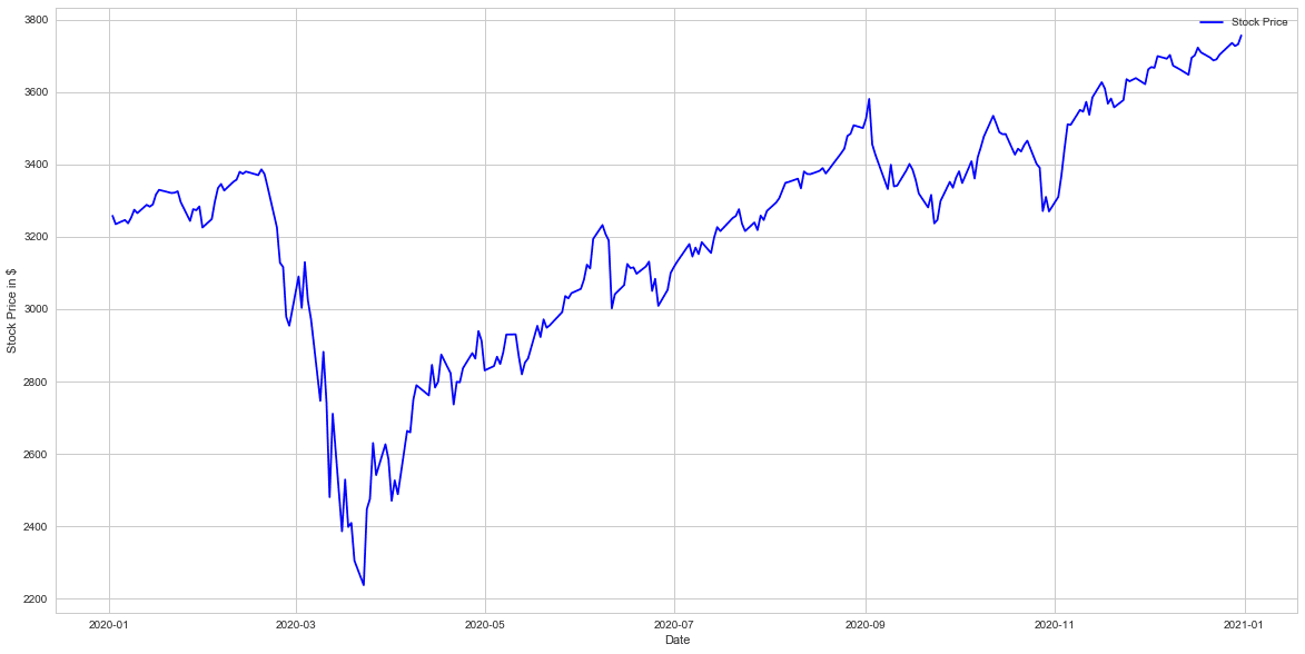
となります。一括投資が分割投資に負けているのは2011年、2014年、2020年、2022年の4年間です。そのうち2011年、2014年、2022年は下げ相場です。2020年はコロナショックのため株価のチャートは下記のような年でした。
この年のパフォーマンスの比較では
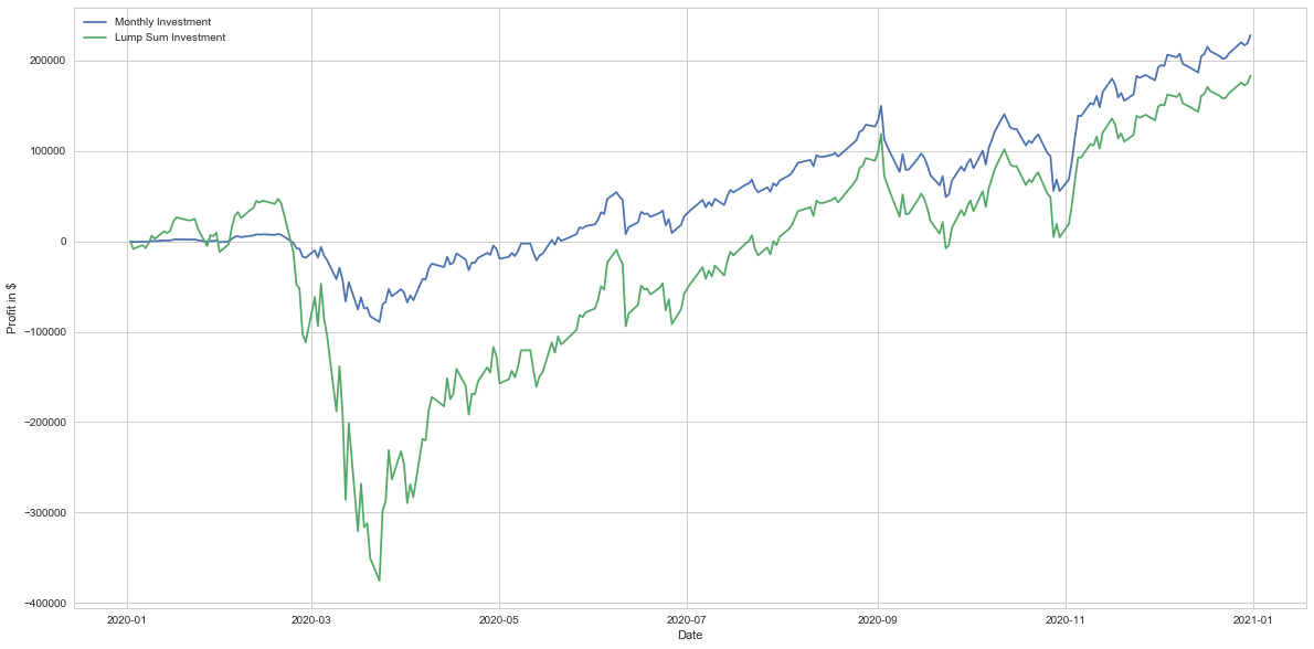
となっており一括投資はコロナの暴落で大きな損益を出しています。2020年のチャートは特殊で大きく下げたあと年末にかけて大きく上がっていっています。このような大暴落があると一括投資は分割投資に負けてしまいます。
資金に余裕があるのであれば一括投資
一般投資家に取って株価は下記のような変動をします。
1) 短期的な株価が予測できない
2) 長期的には上昇が期待できる
この場合は数学的には一番最初にできるだけ購入する、すなわち一括投資が正解です。
一番リターンが大きい=一番たくさん株が買える=最安値で買える、ということですので一番株価が安いのは投資を始めた日である可能性が一番高いです。余剰資金であるのであれば一括投資が一番リターンの期待値が大きいという結論になりました。新NISAも年初の取引初日に全額投資が正解です。私も成長投資枠はオルカンに一括投資しました。
株価は見ない
株価は予想できないのであれば、余剰資金で年初に一括投資、あとは株価を見る必要はありません。毎日株価をみて一喜一憂するのは時間の無駄です。買うタイミングを考えても一番安く変える確率が高いのはいまそのときです。株価をみて買うタイミングを図る時間があれば、その時間を他のことにふりむけるほうが人生は豊かになるのではないでしょうか。