
[Python]健診データ240次元を主成分分析してみた

はじめに
こんにちは、機械学習勉強中のあおじるです。
以前の記事で、医療費データ(160次元)を主成分分析(PCA)してみました。今回は、健診データ(240次元)を主成分分析してみます。
言語はPython、環境はGoogle Colaboratoryを使用しました。
健診データの主成分分析
1.データ
データは、前回の記事で使用した、全国健康保険協会(協会けんぽ)の生活習慣病予防健診の結果の年度、都道府県、性、年齢階級別の時系列データ「健診結果基本情報」を用います。データレイアウトはこちらです。
使用項目
健診項目のうち、2014年度以降しかデータのないHbA1cを除き、また、身長、体重を除いた15個の検査値を用いることにしました。
対象期間
受診控えがあったと思われる2020年度(令和2年度)のデータを除き、2010年度(平成22年度)~2019年度(令和元年度)までの10年分のデータを用いました。
これをデータフレームに読み込み、加工しやすいように以下の形にしておきます。
# データ
import pandas as pd
df_kenshin = pd.read_csv('./健診結果基本情報.csv', encoding='shift_jis')
print(df_kenshin.columns)
# Index(['年度', '都道府県コード', '被保険者被扶養者区分', '性別', '年齢階級',
#        '健診項目', '検査値の合計', '検査人数'], dtype='object')
print(df_kenshin.shape)
# (132352, 8)

df_kenshin = df_kenshin.iloc[:,[0,1,3,4,5,6,7]]
df_kenshin.columns = ['y','t','s','n','k','X','P']
print(df_kenshin.shape)
# (132352, 7)

df_kenshin = df_kenshin.query('not k in ["HbA1c", "身長", "体重"]') \
                       .reset_index(drop=True)
print(df_kenshin.columns)
# Index(['y', 't', 's', 'n', 'k', 'X', 'P'], dtype='object')
print(df_kenshin.shape)
# (112800, 7)

k_ab = {'腹囲': 'WC',
        'BMI': 'BMI',
        '収縮期血圧': 'SBP',
        '拡張期血圧': 'DBP',
        '総コレステロール': 'TC',
        '中性脂肪': 'TG',
        'HDL': 'HDLC',
        'LDL': 'LDLC',
        'GOT': 'GOT',
        'GPT': 'GPT',
        'γGTP': 'yGTP',
        '空腹時血糖': 'FBS',
        '尿酸': 'UA',
        '血清クレアチニン': 'Cr',
        'eGFR': 'eGFR'}
df_kenshin_ab = df_kenshin.copy()
df_kenshin_ab['k'] = [k_ab[df_kenshin.loc[i,'k']] for i in range(len(df_kenshin))]
df_ytsnk_kenshin = df_kenshin_ab.copy()
print(df_ytsnk_kenshin.columns)
# Index(['y', 't', 's', 'n', 'k', 'X', 'P'], dtype='object')
print(df_ytsnk_kenshin.shape)
# (112800, 7)
df_ytsnk_kenshin.to_csv('./df_ytsnk_kenshin.csv', index=None)
$$
\def\arraystretch{1.5}
\begin{array}{c:c:c:c:c|c:c}
\textsf{y} & \textsf{t} & \textsf{s} & \textsf{n} & \textsf{k} & \textsf{X} & \textsf{P} \\ \hline
2010 & 1 & 1 & 1 & \textrm{WC} & {} & {} \\
2010 & 1 & 1 & 2 & \textrm{WC} & {} & {} \\
\vdots & \vdots & \vdots & \vdots & \vdots & \vdots & \vdots \\
2019 & 47 & 2 & 8 & \textrm{eGFR} & {} & {}
\end{array}
$$
y:年度
2010~2019 の10年度分t:都道府県
1:北海道、2:青森、3:岩手、4:宮城、5:秋田、6:山形、7:福島、8:茨城、9:栃木、10:群馬、11:埼玉、12:千葉、13:東京、14:神奈川、15:新潟、16:富山、17:石川、18:福井、19:山梨、20:長野、21:岐阜、22:静岡、23:愛知、24:三重、25:滋賀、26:京都、27:大阪、28:兵庫、29:奈良、30:和歌山、31:鳥取、32:島根、33:岡山、34:広島、35:山口、36:徳島、37:香川、38:愛媛、39:高知、40:福岡、41:佐賀、42:長崎、43:熊本、44:大分、45:宮崎、46:鹿児島、47:沖縄 の47都道府県s:性別
1:男性、2:女性n:年齢階級(5歳階級)
1:35~39歳、2:40~44歳、3:45~49歳、4:50~54歳、5:55~59歳、6:60~64歳、7:65~69歳、8:70歳以上k:健診項目
WC :腹囲 (Waist circumference)(cm)、
BMI :BMI (Body mass index)(kg/m2)、
SBP :収縮期血圧 (Systolic blood pressure)(mmHg)、
DBP :拡張期血圧 (Diastolic blood pressure)(mmHg)、
TC :総コレステロール (Total cholesterol)(mg/dL)、
TG :中性脂肪(血清トリグリセリド) (Triglycerides)(mg/dL)、
HDLC :HDLコレステロール (HDL-cholesterol)(mg/dL)、
LDLC :LDLコレステロール (LDL-cholesterol)(mg/dL)、
GOT :AST(GOT)(U/L)、
GPT :ALT(GPT)(U/L)、
yGTP :γ-GT(γ-GTP)(Gamma-glutamyl transpeptidase)(U/L)、
FBS :空腹時血糖 (Fasting blood sugar)(mg/dL)、
UA :尿酸 (Uric acid)(mg/dL)、
Cr :血清クレアチニン (Creatinine)(mg/dL)、
eGFR:eGFR (estimated GFR)(mL/min)X:検査値の合計
P:検査人数
2.データの加工
年度(y)、都道府県(t)、性(s)、年齢階級(n)及び健診項目(k)ごとに分子(X)と分母(P)から平均値(XperP = X / P)を計算します。
import pandas as pd
df_ytsnk_kenshin = pd.read_csv('./df_ytsnk_kenshin.csv', encoding='shift_jis')
print(df_ytsnk_kenshin.columns)
# Index(['y', 't', 's', 'n', 'k', 'X', 'P'], dtype='object')
print(df_ytsnk_kenshin.shape)
# (112800, 7)

df_ytsn_k_XperP = df_ytsnk_kenshin.copy()
df_ytsn_k_XperP['XperP'] = df_ytsn_k_XperP.X / df_ytsn_k_XperP.P
print(df_ytsn_k_XperP.columns)
# Index(['y', 't', 's', 'n', 'k', 'X', 'P', 'XperP'], dtype='object')
print(df_ytsn_k_XperP.shape)
# (112800, 8)
行方向に並んでいる健診項目(k)を列方向に移します。
df_ytsn_K15 = df_ytsn_k_XperP.copy()
df_ytsn_K15 = df_ytsn_K15.pivot(index=['y','t','s','n'],
                                columns=['k'],
                                values='XperP')
k_names_ab = ['WC', 'BMI', 'SBP', 'DBP', 'TC', 'TG', 'HDLC', 'LDLC',
              'GOT', 'GPT', 'yGTP', 'FBS', 'UA', 'Cr', 'eGFR']
df_ytsn_K15 = df_ytsn_K15.loc[:, k_names_ab]
df_ytsn_K15.set_axis(k_names_ab, axis='columns', inplace=True)
df_ytsn_K15 = df_ytsn_K15.reset_index()
print(df_ytsn_K15.columns)
# Index(['y', 't', 's', 'n', 'WC', 'BMI', 'SBP', 'DBP', 'TC', 'TG', 'HDLC',
#        'LDLC', 'GOT', 'GPT', 'yGTP', 'FBS', 'UA', 'Cr', 'eGFR'],
#       dtype='object')
print(df_ytsn_K15.shape)
# (7520, 19)
# 10*47*2*8=7520, 4+15=19
さらに、性(s)、年齢階級(n)も列方向に移します。
df_yt_K15_sn = df_ytsn_K15.pivot(index=['y','t'],
                                 columns=['s','n'],
                                 values=k_names_ab)
col_names = []
for k_name in k_names_ab:
  for s in [1,2]:
    for n in [1,2,3,4,5,6,7,8]:
      # print(k_name+'_'+str(s)+'_'+str(n))
      col_names.append(k_name+'_'+str(s)+'_'+str(n))
df_yt_K15_sn = df_yt_K15_sn.set_axis(col_names, axis='columns') \
                           .reset_index()
print(df_yt_K15_sn.columns)
# Index(['y', 't', 'WC_1_1', 'WC_1_2', 'WC_1_3', 'WC_1_4', 'WC_1_5', 'WC_1_6',
#        'WC_1_7', 'WC_1_8',
#        ...
#        'eGFR_1_7', 'eGFR_1_8', 'eGFR_2_1', 'eGFR_2_2', 'eGFR_2_3', 'eGFR_2_4',
#        'eGFR_2_5', 'eGFR_2_6', 'eGFR_2_7', 'eGFR_2_8'],
#       dtype='object', length=242)
print(df_yt_K15_sn.shape)
# (470, 242) # 2+15*2*8=242
df_yt_K15_sn.to_csv('./df_yt_K15_sn.csv', index=None)
これで、
(10年×47都道府県)×(15健診項目×性別2区分×年齢階級8区分)
= 470行 × 240次元
の形のデータができました。
$$
\def\arraystretch{1.5}
\begin{array}{c:c|c:c:c:c}
\textsf{y} & \textsf{t} & \textsf{WC\_1\_1} & \textsf{WC\_1\_2} & \cdots & \textsf{eGFR\_2\_8} \\ \hline
2010 & 1 & {} & {} & {} & {} \\
2010 & 2 & {} & {} & {} & {} \\
\vdots & \vdots & \vdots & \vdots & \ddots & \vdots \\
2019 & 47 & {} & {} & {} & {}
\end{array}
$$
y:年度
2010~2019 の10年度分t:都道府県
1:北海道、・・・、47:沖縄 の47都道府県K15_s_n:性別(s)、年齢階級(n)別の15の健診項目の平均値(K15)
K15:15の健診項目(WC、BMI、SBP、DBP、TC、TG、HDLC、LDLC、GOT、GPT、yGTP、FBS、UA、Cr、eGFR)の平均値
s:性別
1:男性、2:女性n:年齢階級
1:35~39歳、2:40~44歳、・・・、7:65~69歳、8:70歳以上
3.PCAの実行
このデータを用いて、PCA(主成分分析)を実行します。
# データ
import pandas as pd
df_yt_K15_sn = pd.read_csv('./df_yt_K15_sn.csv')
print(df_yt_K15_sn.shape)
# (470, 242)

# 数値部分のみ取り出し
df = df_yt_K15_sn.copy()
X = df.iloc[:,2:]
print(X.shape)
# (470, 240)
# 470=10*47, 240=15*2*8
前処理
スケールの異なる健診項目ごとのデータなので、前処理としてスケーリングしておきます。医療費データの場合と同じくMinMaxScalerを使いました。
# スケーリング
from sklearn import preprocessing
scaler = preprocessing.MinMaxScaler()
X = scaler.fit_transform(X)
print(X.shape)
# (470, 240)
PCA
scikit-learnのdecomposition.PCAを使って主成分分析を実行します。
# PCA
from sklearn.decomposition import PCA
pca = PCA()
PC = pca.fit_transform(X)
print(PC.shape)
# (470, 240)
寄与率
累積寄与率を見ると、第8主成分までで8割を超えていました。
import numpy as np
np.set_printoptions(precision=5, suppress=True) # numpyの表示桁数設定
print(pca.explained_variance_ratio_) # 寄与率
# [0.26103 0.16972 0.14162 0.07823 0.06034 0.04703 0.0252  0.02192 0.01722
#  0.01667 0.01444 0.01101 0.01035 0.01021 0.00814 0.00693 0.00647 0.00555
#  0.00514 0.00434 0.00373 0.00352 0.00316 0.00303 0.00288 0.00239 0.00219
#  0.00209 0.00205 0.00196 0.00181 0.00166 0.00159 0.00152 0.00147 0.00139
#  0.00137 0.00131 0.00122 0.00118 0.00114 0.00108 0.00104 0.00102 0.001
#  0.00096 0.00089 0.00086 0.00085 0.00083 0.00078 0.00076 0.00074 0.00073
#  0.00068 0.00067 0.00066 0.00062 0.0006  0.00059 0.00058 0.00055 0.00053
#  0.00051 0.0005  0.00049 0.00048 0.00047 0.00043 0.00042 0.00042 0.00041
#  0.0004  0.00039 0.00038 0.00037 0.00037 0.00035 0.00033 0.00033 0.00032
#  0.0003  0.00029 0.00029 0.00029 0.00028 0.00027 0.00027 0.00026 0.00024
#  0.00024 0.00024 0.00023 0.00022 0.00022 0.00021 0.0002  0.0002  0.00019
#  0.00019 0.00018 0.00018 0.00018 0.00017 0.00016 0.00016 0.00016 0.00015
#  0.00015 0.00015 0.00014 0.00014 0.00013 0.00013 0.00012 0.00012 0.00012
#  0.00012 0.00012 0.00011 0.00011 0.00011 0.00011 0.0001  0.0001  0.0001
#  0.00009 0.00009 0.00009 0.00009 0.00009 0.00008 0.00008 0.00008 0.00008
#  0.00008 0.00007 0.00007 0.00007 0.00007 0.00007 0.00006 0.00006 0.00006
#  0.00006 0.00006 0.00006 0.00006 0.00005 0.00005 0.00005 0.00005 0.00005
#  0.00005 0.00004 0.00004 0.00004 0.00004 0.00004 0.00004 0.00004 0.00004
#  0.00004 0.00003 0.00003 0.00003 0.00003 0.00003 0.00003 0.00003 0.00003
#  0.00003 0.00003 0.00003 0.00002 0.00002 0.00002 0.00002 0.00002 0.00002
#  0.00002 0.00002 0.00002 0.00002 0.00002 0.00002 0.00002 0.00002 0.00002
#  0.00001 0.00001 0.00001 0.00001 0.00001 0.00001 0.00001 0.00001 0.00001
#  0.00001 0.00001 0.00001 0.00001 0.00001 0.00001 0.00001 0.00001 0.00001
#  0.00001 0.00001 0.00001 0.00001 0.00001 0.      0.      0.      0.
#  0.      0.      0.      0.      0.      0.      0.      0.      0.
#  0.      0.      0.      0.      0.      0.      0.      0.      0.
#  0.      0.      0.      0.      0.      0.     ]
print(np.cumsum(pca.explained_variance_ratio_)) # 累積寄与率
# [0.26103 0.43075 0.57236 0.65059 0.71093 0.75796 0.78316 0.80508 0.82229
#  0.83897 0.85341 0.86442 0.87478 0.88498 0.89312 0.90006 0.90653 0.91208
#  0.91722 0.92155 0.92528 0.92881 0.93196 0.93499 0.93787 0.94026 0.94245
#  0.94454 0.94659 0.94855 0.95037 0.95203 0.95362 0.95514 0.95661 0.958
#  0.95937 0.96068 0.9619  0.96308 0.96422 0.9653  0.96634 0.96736 0.96836
#  0.96932 0.97021 0.97108 0.97193 0.97275 0.97354 0.9743  0.97504 0.97577
#  0.97645 0.97712 0.97778 0.97841 0.97901 0.9796  0.98018 0.98073 0.98126
#  0.98178 0.98227 0.98276 0.98324 0.98371 0.98415 0.98457 0.98499 0.9854
#  0.9858  0.9862  0.98658 0.98695 0.98732 0.98766 0.988   0.98832 0.98864
#  0.98894 0.98924 0.98953 0.98982 0.9901  0.99037 0.99064 0.9909  0.99114
#  0.99138 0.99162 0.99184 0.99206 0.99228 0.99249 0.99269 0.99289 0.99308
#  0.99327 0.99345 0.99363 0.99381 0.99398 0.99414 0.9943  0.99445 0.99461
#  0.99476 0.9949  0.99504 0.99518 0.99531 0.99544 0.99557 0.99569 0.99581
#  0.99593 0.99604 0.99616 0.99627 0.99638 0.99648 0.99659 0.99669 0.99679
#  0.99688 0.99697 0.99706 0.99715 0.99724 0.99732 0.9974  0.99748 0.99756
#  0.99763 0.99771 0.99778 0.99785 0.99792 0.99798 0.99805 0.99811 0.99817
#  0.99823 0.99829 0.99835 0.9984  0.99846 0.99851 0.99856 0.99861 0.99866
#  0.9987  0.99875 0.99879 0.99884 0.99888 0.99892 0.99896 0.99899 0.99903
#  0.99907 0.9991  0.99913 0.99917 0.9992  0.99923 0.99926 0.99929 0.99932
#  0.99935 0.99937 0.9994  0.99942 0.99945 0.99947 0.99949 0.99951 0.99954
#  0.99956 0.99958 0.9996  0.99962 0.99963 0.99965 0.99967 0.99969 0.9997
#  0.99972 0.99973 0.99975 0.99976 0.99977 0.99979 0.9998  0.99981 0.99982
#  0.99983 0.99984 0.99985 0.99986 0.99987 0.99988 0.99989 0.99989 0.9999
#  0.99991 0.99991 0.99992 0.99993 0.99993 0.99994 0.99994 0.99995 0.99995
#  0.99995 0.99996 0.99996 0.99996 0.99997 0.99997 0.99997 0.99997 0.99998
#  0.99998 0.99998 0.99998 0.99998 0.99999 0.99999 0.99999 0.99999 0.99999
#  0.99999 1.      1.      1.      1.      1.     ]

%matplotlib inline
import matplotlib.pyplot as plt
plt.figure()
plt.plot(np.cumsum(pca.explained_variance_ratio_)[:40+1], '-o')
plt.xlabel('principal components')
plt.ylabel('cumulative contribution rate')
plt.grid()
plt.show()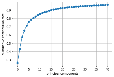
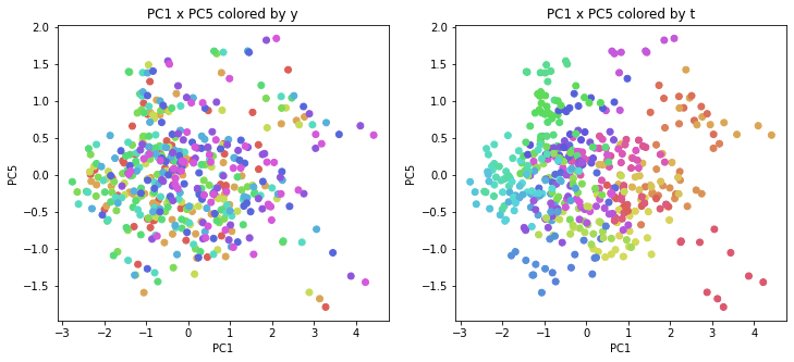
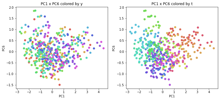
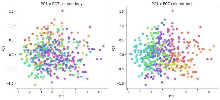
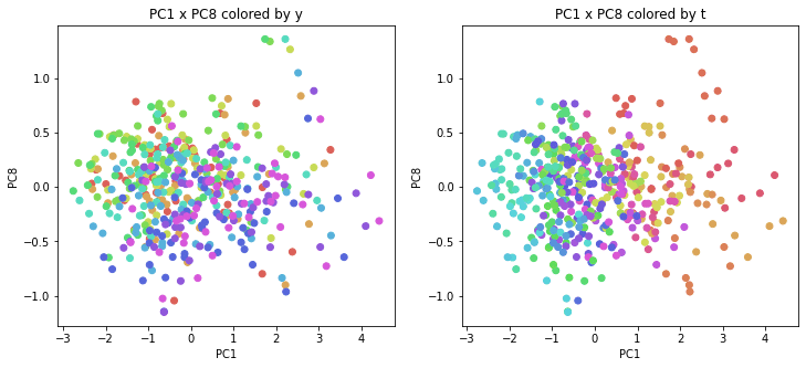
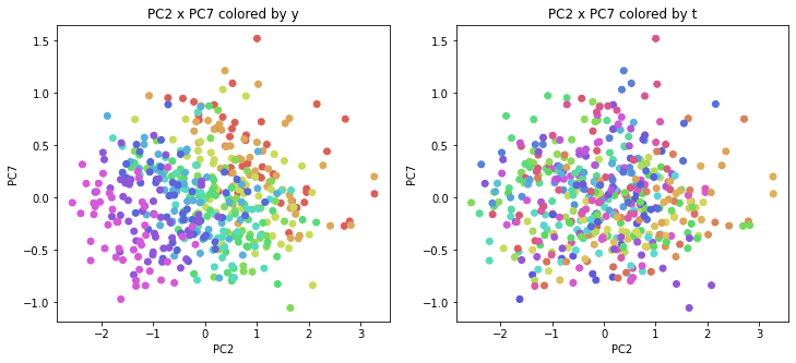
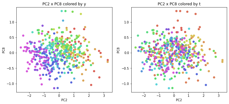
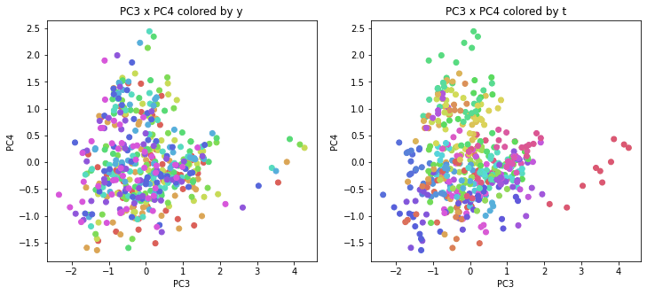
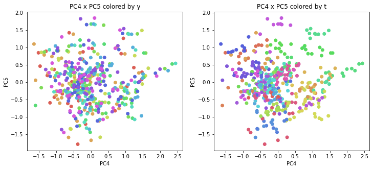
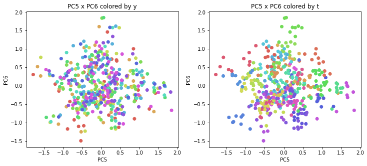
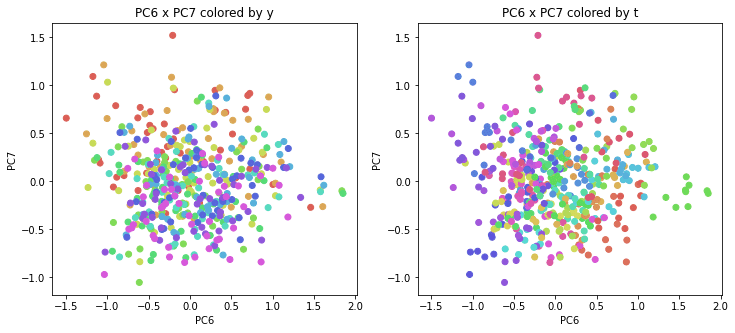
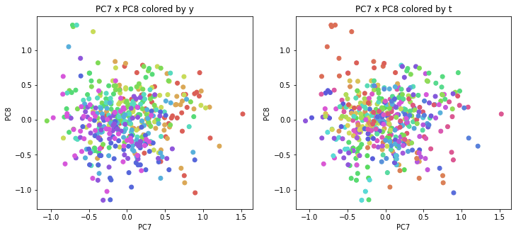
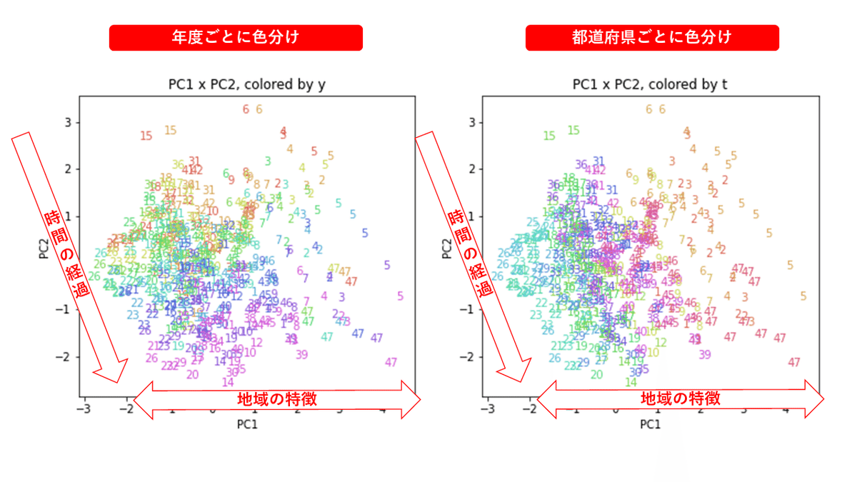
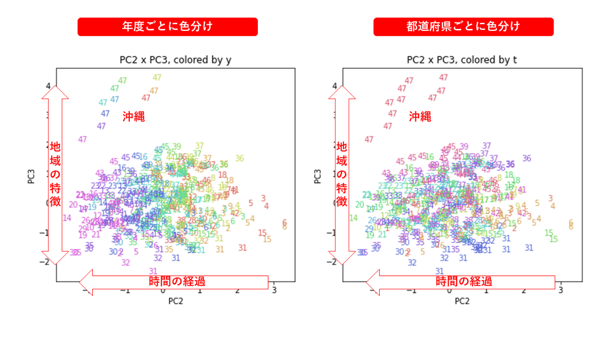
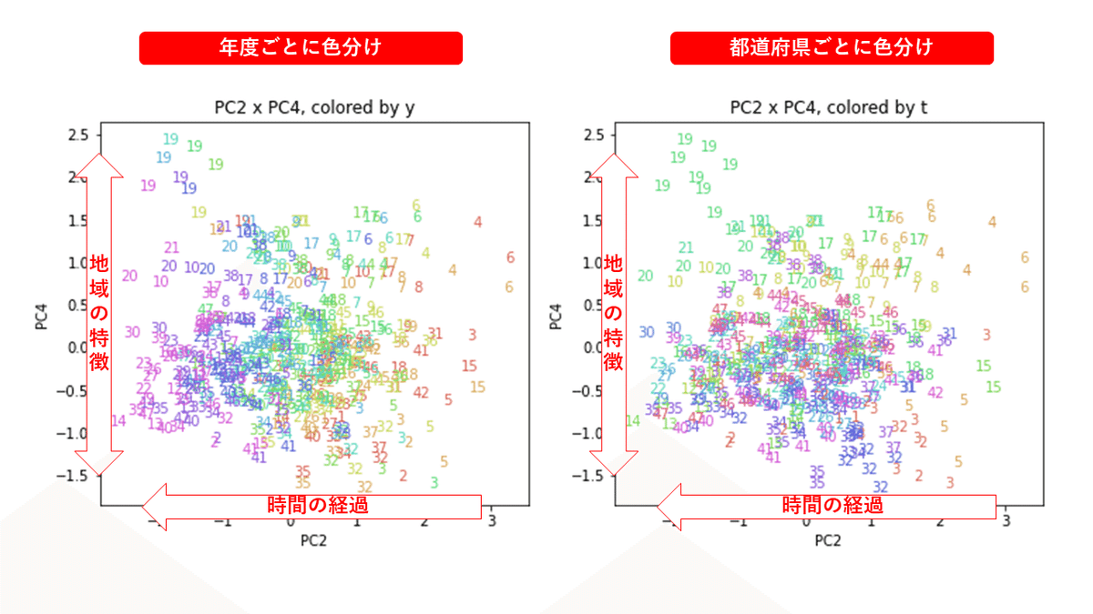
4.結果の図示
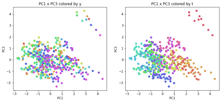
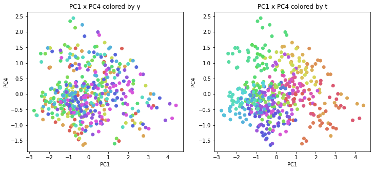
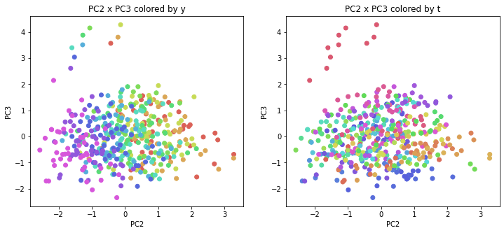
年度別・都道府県別の色分け
PCAの結果の第n主成分をPCnと表記します。
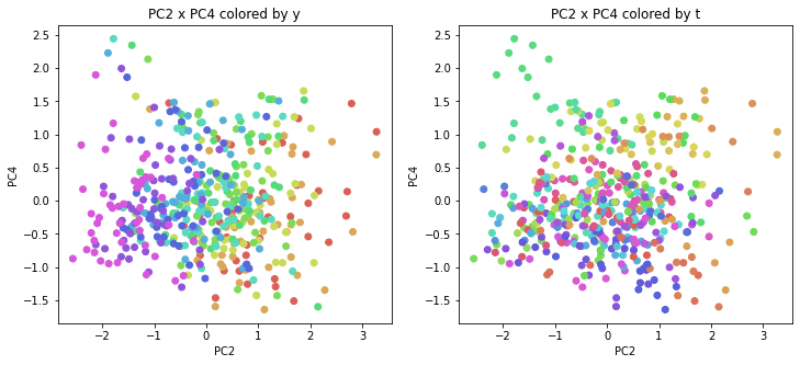
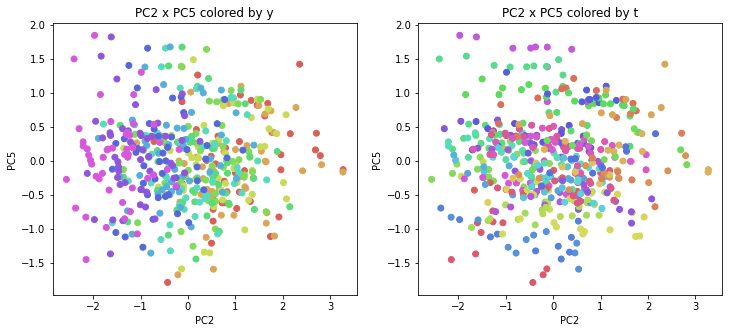
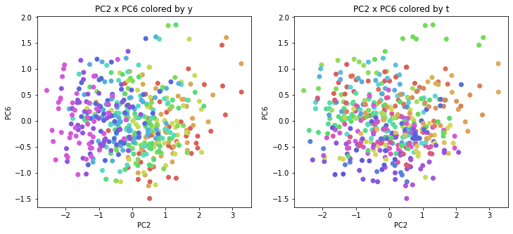
医療費データの場合と同様に、PCAの結果を見やすく表示するため、seabornのカラーパレットを使って、年月別、都道府県別に色分けして図示してみます(左側が年月別に色分け、右側が都道府県別に色分け)。PC1~PC8まで表示しました。
%matplotlib inline
import matplotlib.pyplot as plt
import seaborn as sns
from sklearn import preprocessing
le = preprocessing.LabelEncoder()
# 年度y
label_y = le.fit_transform(df['y'])
cp = sns.color_palette('hls', n_colors=10+1)
color_y = [cp[x] for x in label_y]
# 都道府県t
label_t = le.fit_transform(df['t'])
cp = sns.color_palette('hls', n_colors=47+1)
color_t = [cp[x] for x in label_t]

n = 8
for i in range(n):
  for j in range(i+1,n):
    if (i==0 or i==1 or j==i+1):
      print('PC{} x PC{}'.format(i+1, j+1))
      plt.figure(figsize=(12,5))
      plt.subplot(1, 2, 1)
      plt.title('PC{} x PC{} colored by y'.format(i+1, j+1))
      plt.xlabel('PC{}'.format(i+1))
      plt.ylabel('PC{}'.format(j+1))
      plt.scatter(x=PC[:,i], y=PC[:,j], c=color_y)
      plt.subplot(1, 2, 2)
      plt.title('PC{} x PC{} colored by t'.format(i+1, j+1))
      plt.xlabel('PC{}'.format(i+1))
      plt.ylabel('PC{}'.format(j+1))
      plt.scatter(x=PC[:,i], y=PC[:,j], c=color_t)
      plt.show()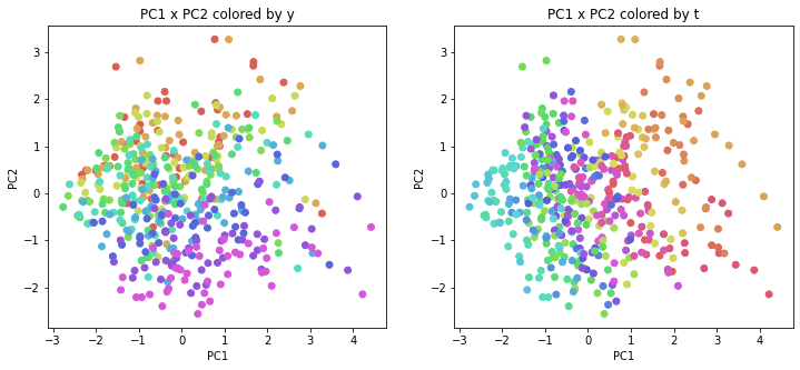
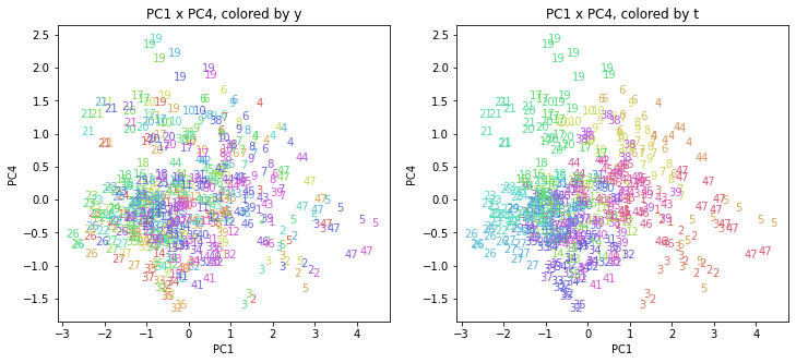
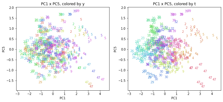
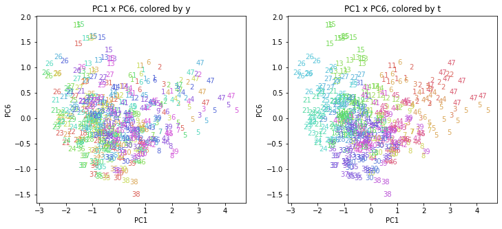
都道府県番号の表示
上の色分けだけでは都道府県が区別しにくいので、医療費データの場合と同様に、点の代わりに都道府県番号をプロットした図も描いておきます(色分けは上と同じ)。
n = 8
for i in range(n):
  for j in range(i+1,n):
    if (i==0 or i == 1 or j==i+1):
      print('PC{} x PC{}'.format(i+1, j+1))
      xmin, xmax = min(PC[:,i]), max(PC[:,i])
      ymin, ymax = min(PC[:,j]), max(PC[:,j])
      plt.figure(figsize=(12,5))
      plt.subplot(1, 2, 1)
      plt.title('PC{} x PC{}, colored by y'.format(i+1, j+1))
      plt.xlabel('PC{}'.format(i+1))
      plt.ylabel('PC{}'.format(j+1))
      plt.xlim(xmin-(xmax-xmin)/20, xmax+(xmax-xmin)/20)
      plt.ylim(ymin-(ymax-ymin)/20, ymax+(ymax-ymin)/20)
      for p in range(len(df)):
        plt.text(x=PC[p,i], y=PC[p,j], s=df.iloc[p,1],
                 ha='center', va='center', fontsize=10, color=color_y[p])
      plt.subplot(1, 2, 2)
      plt.title('PC{} x PC{}, colored by t'.format(i+1, j+1))
      plt.xlabel('PC{}'.format(i+1))
      plt.ylabel('PC{}'.format(j+1))
      plt.xlim(xmin-(xmax-xmin)/20, xmax+(xmax-xmin)/20)
      plt.ylim(ymin-(ymax-ymin)/20, ymax+(ymax-ymin)/20)
      for p in range(len(df)):
        plt.text(x=PC[p,i], y=PC[p,j], s=df.iloc[p,1],
                 ha='center', va='center', fontsize=10, color=color_t[p])
      plt.show()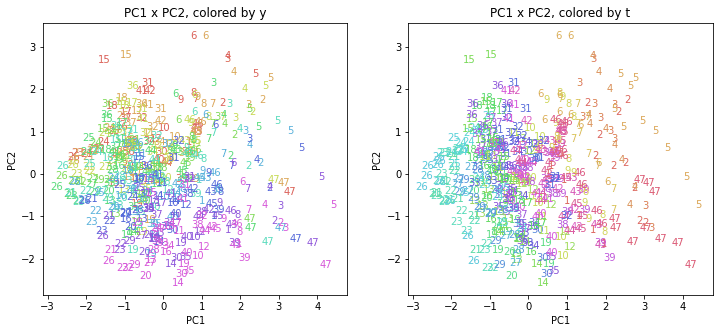
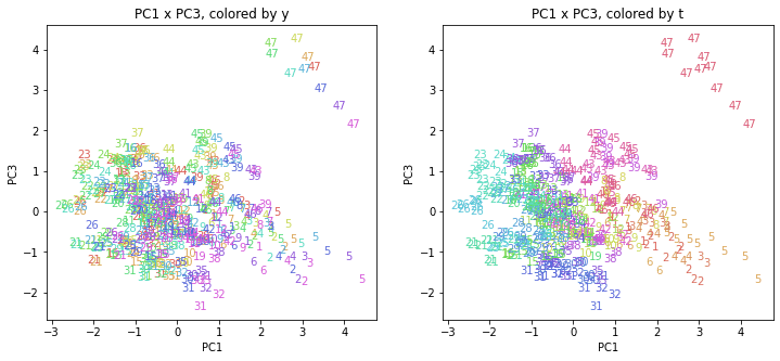

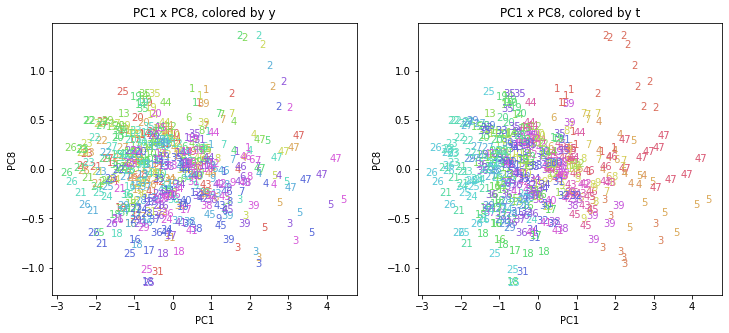
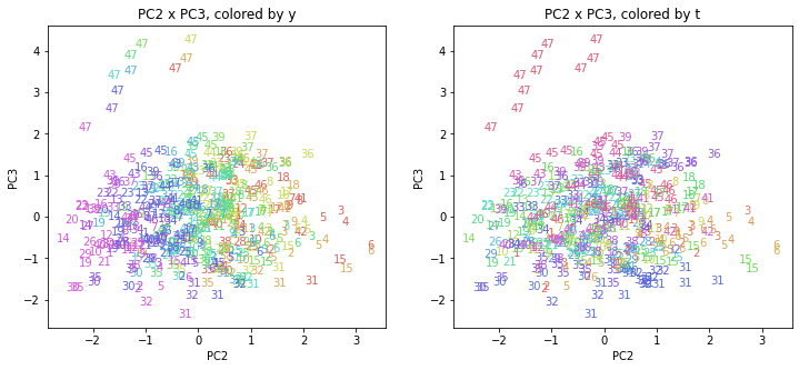
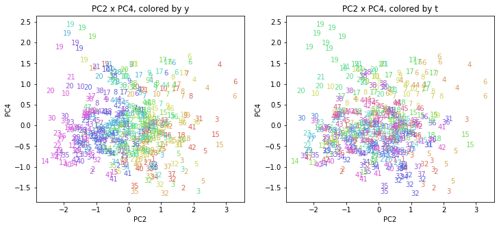
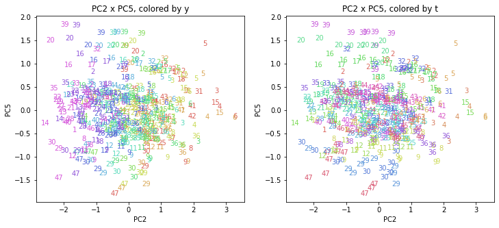
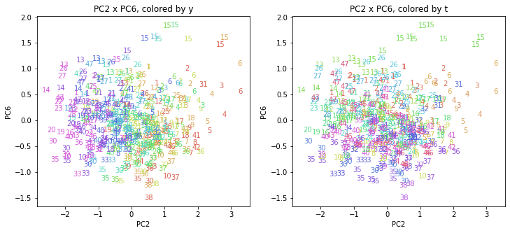
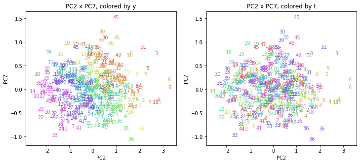
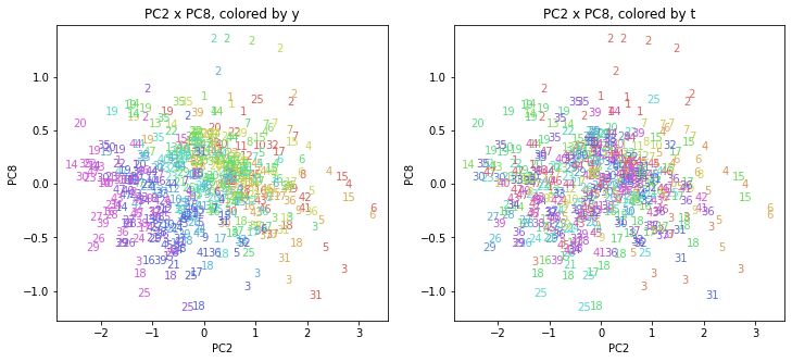
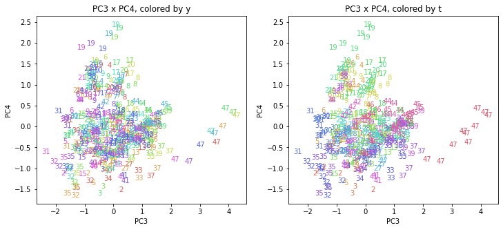
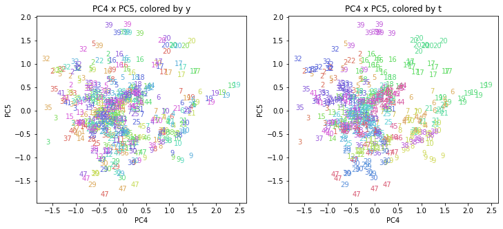
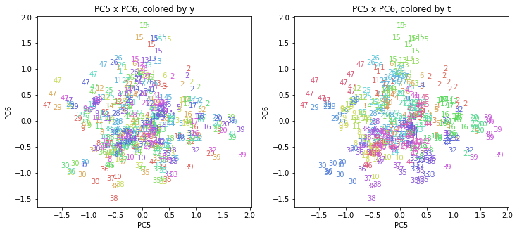
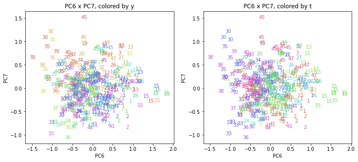
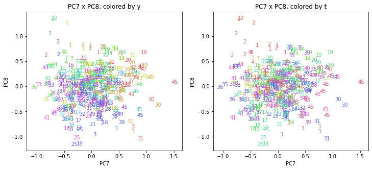
医療費データの場合ほどはっきりとはしていませんが、PC2が概ね時間の経過を表す成分で、残りの成分が時点によって変わらない地域の特徴を表す成分となっているようです。
また、PC1×PC3を見ると、47沖縄が他の都道府県からかなり離れたところに位置しており、沖縄の地域差が際立っているのが分かります。これは、以前別の記事で年齢階級のない健診データでPCAを実行した場合と似た結果となっています。
おわりに
今回は、医療費データと同様に、健診データ240次元についてPCAを実行してみました。PCAの結果、医療費データの場合ほどはっきりしとはしていませんが、第2主成分が概ね時間の経過を表す成分で、時間軸に沿った全体的な動き(全国的な動き)を表しており、それ以外の成分が地域の特徴を表す成分で、この10年間あまり変わっていないことがわかりました。
また、以前別の記事で、年齢階級のない健診データを使ってPCAを実行しましたが、それとも似た結果となりました。
最後まで読んでいただき、ありがとうございました。
お気づきの点等ありましたら、コメントいただけますと幸いです。
#地域差 , #地域間格差 , #都道府県 , #健診 , #健康診断 , #健診項目 , #健診結果 , #健診データ , #生活習慣病予防健診 , #腹囲 , #BMI , #血圧 , #コレステロール , #中性脂肪 , #血糖 , #尿酸 , #肝機能 , #腎機能 , #クレアチニン , #eGFR , #PCA , #次元削減 , #次元 圧縮 , #Python , #協会けんぽ , #noteで数式