
Mapleで制御工学の基礎虎の巻9「状態フィードバック②」

前回の記事では状態フィードバックの意義と状態フィードバックによる固有値配置の方法について説明しました。今回は固有値の配置の仕方による応答の違いについて見ていきましょう。
元のシステムは前回の記事と同じ以下のものとします。

前回の記事でも確認しましたがシステム行列Aの固有値は以下のようになり、正の固有値を持つためシステムは不安定です。

システムのインパルス応答を図1に示しますが、発散してしまっていますね。

さて、このシステムの固有値を前回の記事で説明した固有値配置方法を用いて、以下の3種類の固有値に配置してみましょう。
K1 固有値=[-0.5, -1, -2]
K2 固有値=[-5, -6, -7]
K3 固有値=[-0.5, -1+5i, -1-5i]
K3は前回の記事で配置した固有値ですね。ですから今回はK1とK2の2種類の固有値の振る舞いを追加して、その違いを見てみることにします。
K3は虚数部を持つ固有値でしたが、K1とK2は虚数部を持たず、K1に比べてK2の固有値はより大きな負の値になっています。
この違いが応答にどのような変化をもたらすか実際にインパルス応答を見てみましょう。図2にそれぞれのインパルス応答を示しています。
虚数部のあるK3は振動しているのに、虚数部のないK1とK2は振動が少ないですね。また、固有値がより大きな負の値になっているK1はインパルス応答のピークが小さく、収束も早いですね。これだけ見るとK2、すなわち実数のみでできるだけ負の大きな固有値の方が良いように見えます。ですが本当にそうでしょうか?
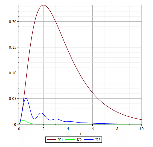
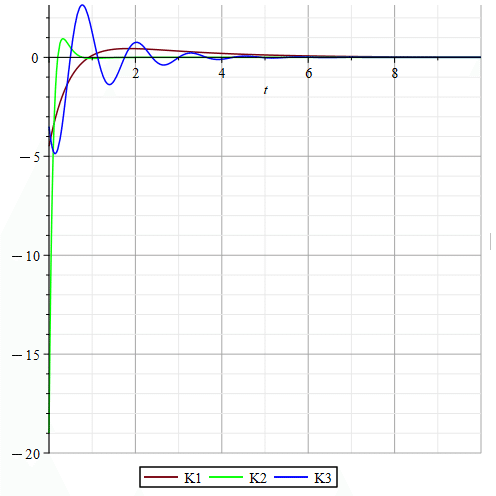
図3にフィードバック入力を示しています。
K2のフィードバック入力はものすごく負の値に振れているのがわかります。K2は出力への影響を抑えられる分、大きな制御エネルギーが必要なことがわかります。一方でK3は振動してしまうもののK1に比べてそんなに大きな制御入力になっていないものの、出力はK1に比べてピークが小さく、収束も早くなっています。
状態フィードバックをする際の固有値の選び方は、期待するシステムの出力の振る舞いだけでなくフィードバック制御入力の大きさも見なければなりません。いかに出力のピークや収束を早めたくても、そのような応答にできる入力を実現できるかわからないからです。制御入力として実現できる範囲になければならないのです。
【English】
In the previous article, we discussed the significance of state feedback and how to place eigenvalues using state feedback. In this article, we will look at the differences in response depending on how the eigenvalues are placed.
The original system should be the same as in the previous article as follows
As confirmed in the previous article, the eigenvalues of the system matrix A are as follows, and the system is unstable because it has positive eigenvalues.
The impulse response of the system is shown in Figure 1, but it has diverged.
Now, let us place the eigenvalues of this system into the following three types of eigenvalues using the eigenvalue placement method described in the previous article.
K1 Eigenvalues=[-0.5, -1, -2]
K2 Eigenvalues=[-5, -6, -7]
K3 Eigenvalues=[-0.5, -1+5i, -1-5i]
K3 is the eigenvalue we placed in the previous article. So this time we will add the behavior of the two eigenvalues, K1 and K2, and see the difference: while K3 was an eigenvalue with an imaginary part, K1 and K2 do not have an imaginary part, and the eigenvalue of K2 is larger and more negative than that of K1.
Let's look at the impulse response to see how this difference changes the response. Figure 2 shows the respective impulse responses.
K3 with the imaginary part is oscillating, while K1 and K2 without the imaginary part are oscillating less. Also, K1, which has a larger negative eigenvalue, has a smaller peak in the impulse response and converges faster. Looking at this only, it seems that K2, i.e., the eigenvalue with only real numbers and as large a negative eigenvalue as possible, is better. But is this really so?
Figure 3 shows the feedback input.
The feedback input of K2 is extremely negative, indicating that K2 requires a large amount of control energy to minimize its output effect. On the other hand, K3, although it oscillates, does not have such a large control input compared to K1, but its output has a smaller peak and converges faster than K1.
When choosing eigenvalues for state feedback, you must look not only at the expected behavior of the system's output, but also at the magnitude of the feedback control input. This is because no matter how much you wish to reduce the peak of the output or to speed up convergence, you do not know if you can achieve an input that will allow you to achieve such a response. The control input must be within the range that is feasible.
【Sample】
Created by Maple 2024.1