予算0円で自動反応経路探索(AFIR)を実装する:④Pythonによる実装

前回までの記事において、AFIRによる自動反応経路探索のアルゴリズム概要と、検証に用いる実例について、それぞれ概要を紹介してきました。本記事ではいよいよ、AFIR(Artificial Force Induced Reaction)法を用いた自動反応経路探索アルゴリズムをPythonスクリプトで実装する方法を紹介します。この実装では、ASE(Atomic Simulation Environment)を用いて構造最適化を行い、反応経路の探索と反応ネットワークの構築を実現します。記事の内容を順を追って説明しながら、コードの各部分を解説していきます。この記事を読んでいただくと、AFIRが非常に自然なアイデアに基づく「ヒューリスティック」な手法であることがよくわかるかと思います。
※なお本記事は、趣味でマテリアルズインフォマティクスを楽しむ兼業主夫の片手間による戯言である以上、実装はかなりプリミティブになる点をご容赦ください(本記事群でお伝えしたいことは、アルゴリズムの再現度や実装の出来不出来といった「枝葉末節」にはございません…これまた界隈の方々を激怒させる文言で恐縮ですが)。
1. AFIR 法の概要
AFIR 法は、人工的な力を特定の原子ペアに適用し、反応経路を探索する手法です。この力は特定のパラメータ γ\gamma に基づいて距離依存で計算されます。探索の過程で力を適用した構造最適化を繰り返し行い、反応ネットワークを構築します。前回の記事を参考にアルゴリズムのステップを復習しますと、以下のようになります。
初期構造の準備
分子系の初期構造を用意します。人工力の設定
“結合を形成・解離させたい”と考える原子対(あるいは分子対)を指定し、その方向に対して人工的な力を加えます。反応経路の探索
仮想力をかけた状態で分子構造を最適化し、エネルギーが下がる方向に反応が進むように計算します。すると、新たな構造や、従来の手法では気づかなかった可能性のある遷移状態が見つかります。人工力の除去
人工力を段階的に小さくしながら、最終的に通常のPES上へ戻します。これにより、“現実的”なエネルギー面での局所極小や遷移状態として確定されます。複数の反応パス探索
上記の操作を複数の原子対・分子対に対して行うことで、多彩な反応パスウェイを同時に洗い出します。手動で行うと膨大な手間がかかる作業ですが、AFIR法によって計算が自動化されるため、大幅な時間短縮や網羅性の向上が期待できます。
2. 実装
以下のスクリプトは、AFIR 法に基づいて自動反応経路を探索するためのフレームワークを実装したものです。
2-1 初期構造の入手
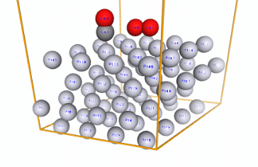
今回は文献のデータを再現するため、以下の構造を作成し、OMat24(31M)にて最適化を行いました(スクリプトは割愛しますが、場合によってはGithubでの公開を検討)。
2-2 人工力の設定
import numpy as np
import networkx as nx
from ase.geometry import get_distances
from ase.optimize import BFGS, FIRE
from copy import deepcopy
import random
import gc
上記のライブラリには、ASE を中心に数値計算(NumPy)やグラフ構築(NetworkX)用のツールが含まれています。グラフ構築用のライブラリは、反応探索時に各パスを管理するために使用します(こんなところで本業で使うライブラリと再会)。
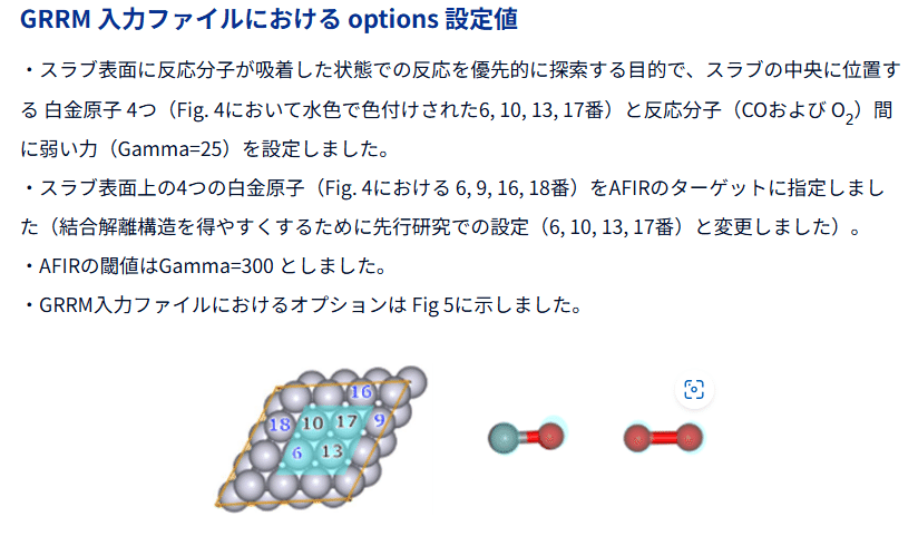
続いて、人工力を印加する結合ペアを設定します。今回は文献および、これをNNPにて再現した検討(GRRM20 With Matlantis 適用事例 - MATLANTIS)を参考に、以下の結合間に人工力を印加することにしました。ここはかなり重要な所でして、AFIRにおいては自然かつ効率的に「あり得そうな反応」を誘起するため、実際に相互作用しそうな結合間に人工力を与え、分子の形状を安定構造から外すという操作が行われます。この「相互作用しそう」という部分は2025年1月現在、人類が行っていますので、まだ完全に手放しでの探索というわけにはいきません(本手法がヒューリスティックである所以、その一です)。
# 弱い力 (Gamma = 25) の対象
weak_force_pt = [35, 40, 58]  # Pt原子
co_indices = [65, 64]         # CO
o2_indices = [66, 67]         # O2

# 強い力 (Gamma = 300) の対象
strong_force_pt = [36, 47, 34, 57, 64, 65, 66, 67]  # Pt原子

# (1) 弱い力のペア
weak_force_pairs = []
for pt in weak_force_pt:
    for reactive in co_indices + o2_indices:
        weak_force_pairs.append((pt, reactive))

# (2) 強い力のペア
strong_force_pairs = []
for i, pt1 in enumerate(strong_force_pt):
    for pt2 in strong_force_pt[i+1:]:
        if pt1 != pt2:
            strong_force_pairs.append((pt1, pt2))

# 結果の表示
print("弱い力のペア (Gamma = 25):", weak_force_pairs)
print("強い力のペア (Gamma = 300):", strong_force_pairs)
実装は上記となります。この部分では、弱い力および強い力を適用する原子ペアを定義しています(強い力だけでなく、弱い力も同時に加えることにより、より多様な構造を生成するという意図)。これにより、AFIR 法が適用される原子対のリストが生成されます。
引き続き、人工力を印加した力場を設定します。何やら高度なクラスに見えますが、要するにやっていることは「既存のcalculatorで計算した力にたいし、特定の結合ペアにのみ人工力を足して出力する」のみです(のみといいつつ、そもそも反応まで取り扱えて、かつ現実的な時間で収束する超高速かつ高精度なニューラルネットワークポテンシャルがない限り、こんなものを趣味で実装しようと思う人は現れなかったでしょう。それが出来てしまったというのが2024年末なのです…タダで)。
class AFIRMCalculator(Calculator):
    implemented_properties = ['energy', 'forces']

    def __init__(self, atoms, atom1, atom2, atom3, atom4, gamma_weak, gamma_strong, original_calc):
        super().__init__()
        self.atoms = atoms
        self.atom1 = atom1
        self.atom2 = atom2
        self.atom3 = atom3
        self.atom4 = atom4
        self.gamma_weak = gamma_weak
        self.gamma_strong = gamma_strong
        self.original_calc = original_calc

    def calculate(self, atoms=None, properties=['energy'], system_changes=all_changes):
        super().calculate(atoms, properties, system_changes)

        # オリジナルのエネルギーと力を取得
        self.original_calc.calculate(self.atoms, properties, system_changes)
        energy = self.original_calc.results['energy']
        forces = self.original_calc.results['forces']

        # 距離に基づく人工力の計算(弱い力)
        positions = self.atoms.get_positions()
        R_weak = positions[self.atom2] - positions[self.atom1]
        distance_weak = np.linalg.norm(R_weak)
        force_magnitude_weak = self.gamma_weak / distance_weak**2
        direction_weak = R_weak / distance_weak

        afir_energy_weak = self.gamma_weak / distance_weak
        afir_force_weak = force_magnitude_weak * direction_weak

        forces[self.atom1] -= afir_force_weak
        forces[self.atom2] += afir_force_weak

        # 距離に基づく人工力の計算(強い力)
        R_strong = positions[self.atom4] - positions[self.atom3]
        distance_strong = np.linalg.norm(R_strong)
        force_magnitude_strong = self.gamma_strong / distance_strong**2
        direction_strong = R_strong / distance_strong

        afir_energy_strong = self.gamma_strong / distance_strong
        afir_force_strong = force_magnitude_strong * direction_strong

        forces[self.atom3] -= afir_force_strong
        forces[self.atom4] += afir_force_strong

        self.results['energy'] = energy + afir_energy_weak + afir_energy_strong
        self.results['forces'] = forces
2-3 反応経路の探索 / 人工力の除去
さらに引き続き、上記の人工力を用いて構造最適化する関数を実装します。アルゴリズムの概要で述べたとおり、AFIRにおいては初めに人工力を印加した後、人工力を排して再度構造最適化することにより、元々の構造から少し離れた新たな局所最適な構造を探索します。今回はこれを、MDに似た最適化手法であるFIREにて、人工力ありの構造最適化を暫く行い、そのあとにもとの力場で再度構造最適化する、という手順にて簡易的に実装しました(実装をみればわかる通り、どのように人工力を取り除くかというのはヒューリスティックその二の構成要素です)。
def apply_afir_force_with_fire(atoms, weak_force_pairs, strong_force_pairs, gamma_weak, gamma_strong, calc_class, steps_with_force=20):
    atoms_copy = deepcopy(atoms)
    atoms1, atoms2 = weak_force_pairs[0], weak_force_pairs[1]
    atoms3, atoms4 = strong_force_pairs[0], strong_force_pairs[1]

    combined_forces = AFIRMCalculator(atoms_copy, atoms1, atoms2, atoms3, atoms4, gamma_weak, gamma_strong, calc_class)
    atoms_copy.calc = combined_forces

    fire_optimizer = FIRE(atoms_copy, logfile=None)
    fire_optimizer.run(fmax=0.1, steps=steps_with_force)

    calc_without_force = calc_class
    atoms_copy.calc = calc_without_force

    optimizer = BFGS(atoms_copy, logfile=None)
    optimizer.run(fmax=0.1, steps=300)

    del optimizer
    gc.collect()

    return atoms_copy
2-4 複数の反応パス探索
それでは、上記の関数群を用いて、複数の反応パス探索を行います。すなわち、どの結合ペアに対して人工力を印加するかという組合せを様々に試しながら、次々と新たな構造を遷移して、どこにたどり着くかを追っていきます。
def iterative_afir_with_network(mol_on_slab, weak_force_pairs, strong_force_pairs, initial_gamma, calc_instance, max_iterations=10, decay_factor=0.9, tolerance=0.15, max_combinations=5, max_structures=10, force_threshold=0.1):
    """
    Perform iterative AFIR process with pruning and network construction.

    Parameters:
        mol_on_slab (ase.Atoms): Initial structure.
        weak_force_pairs (list of tuples): Atom pairs for weak forces.
        strong_force_pairs (list of tuples): Atom pairs for strong forces.
        initial_gamma (float): Initial gamma value.
        max_iterations (int): Maximum number of iterations.
        decay_factor (float): Factor to decay gamma.
        tolerance (float): Tolerance for pruning duplicates.
        max_combinations (int): Maximum number of random pair combinations.
        max_structures (int): Maximum number of stable structures to retain.
        force_threshold (float): Minimum force threshold for appending new structures.

    Returns:
        networkx.DiGraph: Directed graph representing the reaction network.
    """

    all_structures = [mol_on_slab]
    graph = nx.DiGraph()
    mol_on_slab.calc = calc

    # Add the initial structure as the starting node
    graph.add_node(0, structure=mol_on_slab, energy=mol_on_slab.get_potential_energy())

    node_counter = 1

    for iteration in range(max_iterations):
        current_gamma_weak = update_gamma(initial_gamma, iteration, decay_factor)
        current_gamma_strong = current_gamma_weak * 12
        print(f"Iteration {iteration + 1}: Gamma Weak = {current_gamma_weak}, Gamma Strong = {current_gamma_strong}")

        new_structures = []

        for structure_index, structure in enumerate(all_structures):
            print(f"Processing structure {structure_index + 1}/{len(all_structures)}")

            random_combinations = random.sample(
                [(w, s) for w in weak_force_pairs for s in strong_force_pairs],
                min(max_combinations, len(weak_force_pairs) * len(strong_force_pairs))
            )

            for combination_index, (weak_pair, strong_pair) in enumerate(random_combinations):
                print(f"  Combination {combination_index + 1}/{len(random_combinations)}: Weak pair {weak_pair}, Strong pair {strong_pair}")

                new_structure = apply_afir_force_with_fire(
                    structure,
                    weak_pair,
                    strong_pair,
                    current_gamma_weak,
                    current_gamma_strong,
                    calc_instance
                )

                # Check forces to determine if the structure is converged
                forces = new_structure.get_forces()
                max_force = np.max(np.linalg.norm(forces, axis=1))
                print(max_force)
                if max_force < force_threshold:
                    parent_energy = graph.nodes[structure_index]['energy']
                    child_energy = new_structure.get_potential_energy()
                    energy_difference = child_energy - parent_energy

                    new_structures.append(new_structure)
                    graph.add_node(node_counter, structure=new_structure, energy=child_energy)
                    graph.add_edge(structure_index, node_counter, weight=energy_difference)
                    node_counter += 1
                else:
                    print(f"  Skipped structure due to high forces (max force = {max_force})")

        all_structures.extend(new_structures)

        # Retain only the most stable structures based on energy, but keep the initial structure
        all_structures = [mol_on_slab] + sorted(all_structures[1:], key=lambda x: x.get_potential_energy())[:max_structures - 1]

        # Prune duplicates and log reasons
        unique_structures = []
        for structure in all_structures:
            is_duplicate = False
            for unique_structure in unique_structures:
                if is_structure_similar(structure, unique_structure, tolerance):
                    is_duplicate = True
                    print(f"  Pruned structure due to similarity with another structure (Energy: {structure.get_potential_energy():.2f})")
                    break
            if not is_duplicate:
                unique_structures.append(structure)

        all_structures = unique_structures

    return graph
ただし、単に構造を次々生成するだけでは、ステップを増すごとに(iterationが増えるごとに)構造の数が組合せ爆発的に増加してしまいます。そこで、各ステップにて生成する構造の数は多くとりつつ、重複する構造は削除し、またforceが収束していないものも削除し、さらにエネルギー的に安定な構造上位n種に絞る、という形で、次のステップに進められる構造の数を絞るという仕組みにしました。これにより、組合せ爆発を避けつつ多様な構造を探索することが可能となります(ヒューリスティック…! ちなみに私はGAが好きです。知人にはSA派が多く、若干寂しさを覚えます)。
2-5 最適経路の選出
def find_optimal_path(graph):
    """
    Find the path with the minimum energy in the reaction network.

    Parameters:
        graph (networkx.DiGraph): Reaction network graph.

    Returns:
        list: Optimal path as a list of node indices.
    """
    start_node = 0
    end_nodes = [node for node in graph.nodes if graph.out_degree(node) == 0]

    optimal_path = None
    optimal_energy = float('inf')

    for end_node in end_nodes:
        try:
            path = nx.shortest_path(graph, source=start_node, target=end_node, weight='weight')
            path_energy = sum(graph[u][v]['weight'] for u, v in zip(path[:-1], path[1:]))
            if path_energy < optimal_energy:
                optimal_energy = path_energy
                optimal_path = path
        except nx.NetworkXNoPath:
            continue

    return optimal_path
find_optimal_path 関数は、反応ネットワークからエネルギー的に最適な経路を探索します(これはあくまで一例で、実際にはもっと丁寧にパスを選出する必要があります)。
3. 次回予告
次回の記事では、これらのスクリプトを用いた実際の構造探索や、結果の可視化について解説します!