【Python】張力+重力による円錐振子運動

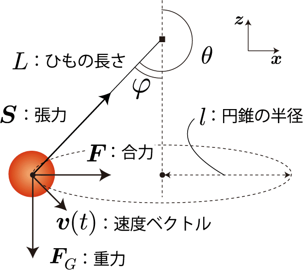
前回紹介した張力+重力による運動は単振り子運動だったけれども、特定の初期条件を与えるとおもりは同一円周上を等速円運動するよ。これは振り子のひもとおもりの軌跡が円錐状になることから円錐振子運動って呼ばれるね。円錐振子運動の理解に必要な量を図示したのが下図だよ。おもりに加わる力は単振子運動と同じだね。
円錐振子運動が実現する条件
円錐振子運動は特定の初期条件の場合のみ実現されるね。その条件は次の2つだよ。
(1)張力と重力の合力が円周軌道平面方向を向く
→ $${\boldsymbol{F}\cdot \hat{z} = 0}$$
(2)張力と重力の合力が等速円運動を実現する遠心力と一致する
→ $${|\boldsymbol{F}| = ml\omega^2}$$
$${l =L\sin\varphi}$$、$${v =l\omega= L\omega \sin\varphi }$$、$${ |F| = S\sin\varphi }$$ を考慮すると先の2つの条件は次のように表されるね。
$$
S\cos\varphi=mg
$$
$$
S\sin\varphi=m\,\frac{v^2}{L\sin\varphi}
$$
この式から円錐振子運動するための速度の大きさの条件は次のとおりに得られるよ。
【解析解】円錐振子運動の速度の大きさ
$$
v=\pm\sqrt{\frac{gL\sin^2\varphi}{\cos\varphi}}
$$
ここまで明示的に言及していませんが(1)と(2)の条件には速度ベクトルが円周軌道の接線方向を向いていることも含まれているよ。つまり、速度ベクトルが円周軌道の接線方向かつ大きさが上式の場合のみ円錐振子運動となるね。一度円錐振子運動が実現されると、外部からおもりに力が加わらない限り円錐振子運動を続けるため、初期条件として上記の条件を満たす必要があるよ。
計算結果
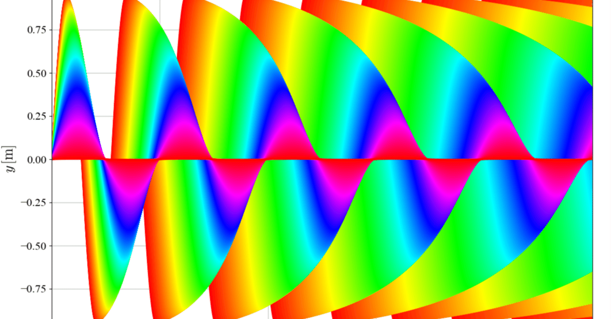
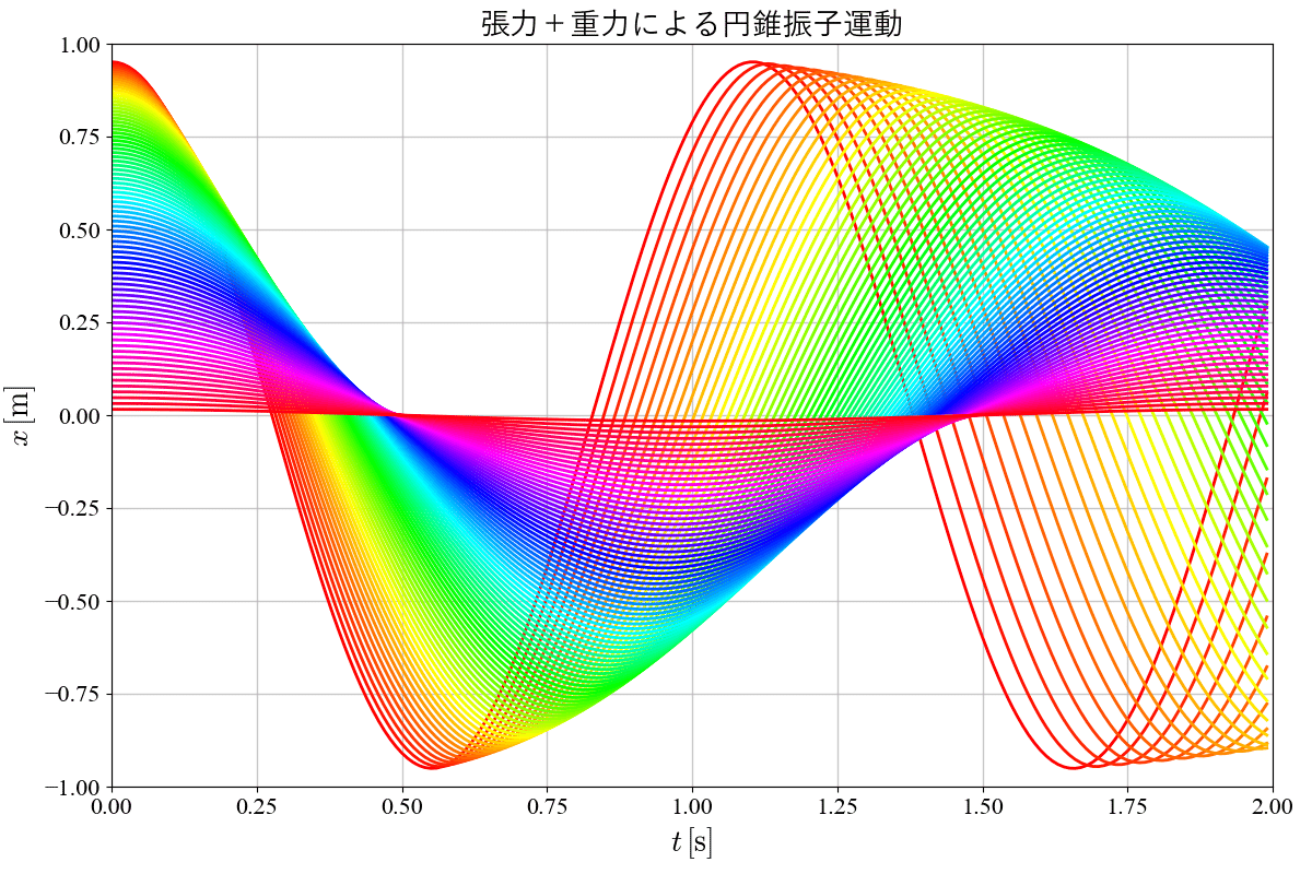
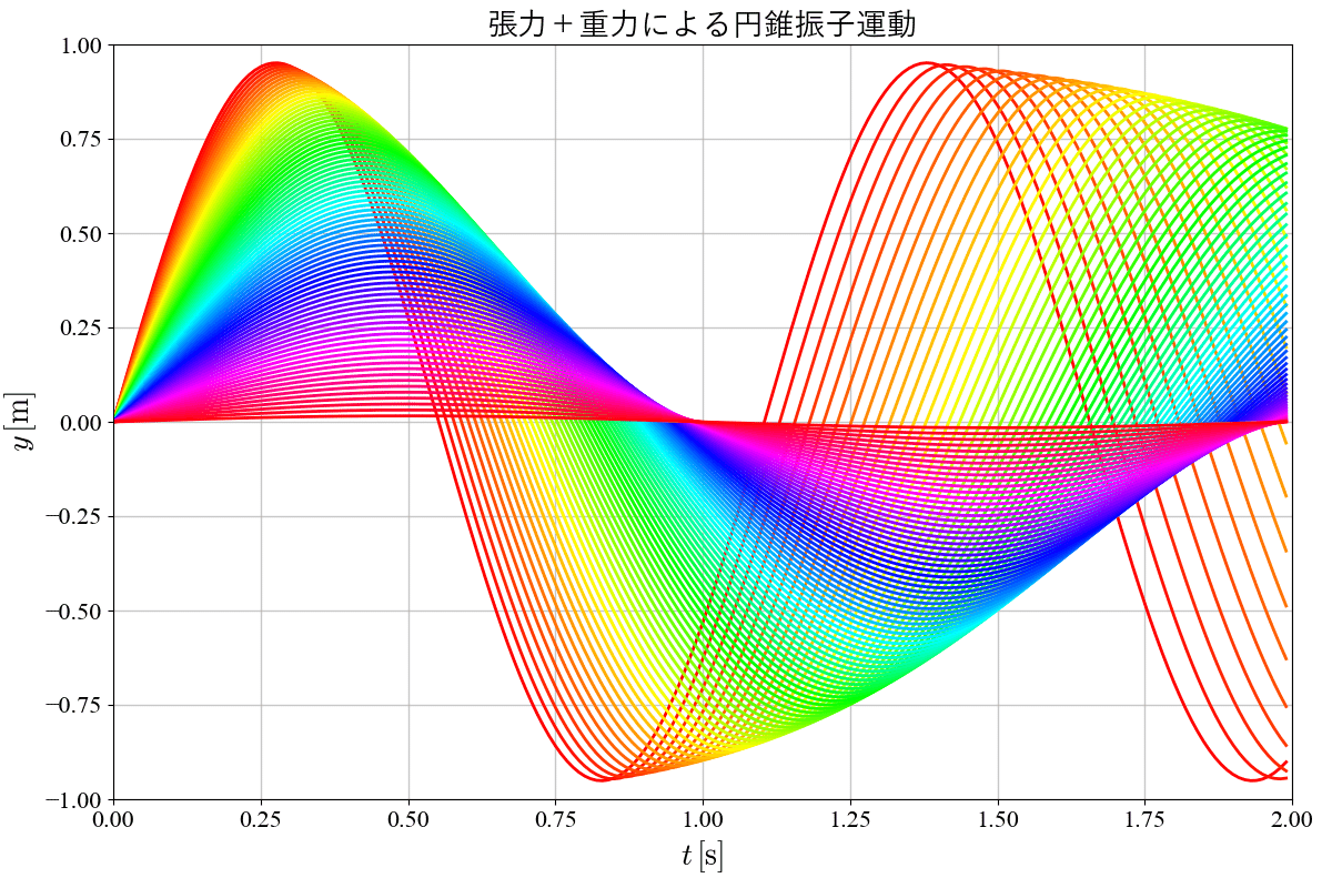
次のグラフはひもの長さ$${L=1}$$、初期位置$${y=0}$$で、偏角$${\varphi}$$を$${0\sim \pi/2}$$まで変化させたときのおもりのx成分とy成分の時間依存性をそれぞれプロットした結果だよ。等速円運動となるので、軌跡は三角関数で表すことができるよ。
Pythonプログラムソース
Pythonプログラムソースを紹介するよ。もし良かったら試してみてください。
#################################################################
TITLE = "張力+重力による円錐振子運動"
#################################################################
import os
import numpy as np
import scipy.integrate as integrate
import matplotlib.pyplot as plt
import matplotlib.animation as animation
import colorsys
###############################
# 実験室グローバル変数
###############################
TIME_START = 0.0        #計算開始時刻
TIME_END   = 2.0       #計算終了時刻
DT = 0.01               #時間間隔
PLOT_FLAG = True        #グラフ描画
ANIMATION_FLAG = False  #アニメーション作成
ANIMATION_INTERVAL = 1 #アニメーション作成時の描画インターバル
OUTPUT_FLAG = False
OUTPUT_PASS = "./data_20240922/"
if( OUTPUT_FLAG and os.path.isdir(OUTPUT_PASS) == False) : os.mkdir(OUTPUT_PASS)
###############################
# 計算グローバル変数
###############################
#時刻
times = np.arange(TIME_START, TIME_END, DT)
#重力加速度
vec_g = np.array([0, 0, -10])
#質量
m = 1.0
#粘性係数
gamma = 0.0
#ひもの長さ
L0 = 1
#初期速度
vec_v0 = np.array([0, 0, 0])
#初期角度
thetas = np.arange(1.2, 2.0, 0.01) * np.pi / 2.0
###############################
# 関数定義
###############################
#張力+重力の微分方程式
def equations(t, X , vec_g, m, compensationK, compensationGamma):
	vec_r =  np.array([ X[0], X[1], X[2] ])
	vec_v =  np.array([ X[3], X[4], X[5] ])
	#紐の長さ
	L = np.sqrt( np.dot(vec_r, vec_r) )
	#速度の大きさ
	v = np.sqrt( np.dot(vec_v, vec_v) )
	#張力
	vec_S = - m / L**2 * ( v**2 + np.dot(vec_g, vec_r) ) * vec_r
	#位置ベクトルと速度ベクトルの単位ベクトル
	hat_r = vec_r / L
	if( v > 0 ): hat_v = vec_v / v
	else: hat_v = vec_v * 0
	#補正力
	f_c = - compensationK * ( L - L0 ) * hat_r - compensationGamma * np.dot(hat_v, hat_r) * hat_r
	#質点に加わる力
	F = vec_S + m * vec_g + f_c * np.sqrt( np.dot(vec_S, vec_S) )
	#ニュートンの運動方程式
	vec_a = F / m
	return [vec_v[0], vec_v[1], vec_v[2], vec_a[0], vec_a[1], vec_a[2]]

# theta 依存性を可視化
def calculation(vec_r0, vec_v0, compensationK, compensationGamma ):

	solution = integrate.solve_ivp(
		equations,                     #常微分方程式
		method = 'RK45',                #計算方法
		args = (vec_g, m, compensationK, compensationGamma),              #引数
		t_span=( times[0], times[-1]),  #積分区間
		rtol = 1.e-5,                   #相対誤差
		atol = 1.e-5,                   #絶対誤差
		y0 = np.concatenate([vec_r0, vec_v0]), #初期値
		t_eval = times                  #結果を取得する時刻
	)
	#計算結果
	return solution.y[ 0 ], solution.y[ 1 ], solution.y[ 2 ], solution.y[ 3 ], solution.y[ 4 ], solution.y[ 5 ]

##########################################################
if __name__ == "__main__":

	#描画用リスト
	xls = []
	yls = []
	zls = []
	vxls = []
	vyls = []
	vzls = []
	#theta による違い
	for i in range(len(thetas)):
		print( i )
		theta = thetas[ i ]
		varphi = theta - np.pi

		g = np.sqrt( np.dot(vec_g, vec_g) )
		v0 = np.sqrt( g * L0 * np.sin( varphi )**2 / np.cos( varphi ) )

		#初期位置と速度
		vec_r0 = np.array([ L0 * np.sin( theta ), 0, L0 * np.cos( theta )])
		vec_v0 = np.array([ 0, v0, 0])

		x, y, z, vx, vy, vz = calculation( vec_r0, vec_v0, 0.3, 0.5 )
		xls.append( x )
		yls.append( y )
		zls.append( z )
		vxls.append( vx )
		vyls.append( vy )
		vzls.append( vz )

	if( OUTPUT_FLAG ):
		for i in range(len(times)):
			path = OUTPUT_PASS + str( i ) + '.txt'
			f = open(path, 'w')

			for j in range( len(xls) ):
				f.write( str(xls[ j ][ i ]) + "\t" +  str(yls[ j ][ i ]) + "\t" + str(zls[ j ][ i ]) + "\t" +  str(vxls[ j ][ i ]) + "\t" + str(vyls[ j ][ i ]) + "\t" +  str(vzls[ j ][ i ]) + "\n")

			f.close()

	if( PLOT_FLAG ):
		#################################################################
		# グラフの設定
		#################################################################
		fig = plt.figure( figsize=(12, 8) ) #画像サイズ
		plt.subplots_adjust(left = 0.085, right = 0.97, bottom = 0.10, top = 0.95) #グラフサイズ
		plt.rcParams['font.family'] = 'Times New Roman' #フォント
		plt.rcParams['font.size'] = 16 #フォントサイズ
		plt.rcParams["mathtext.fontset"] = 'cm' #数式用フォント
		#カラーリストの取得
		colors = plt.rcParams['axes.prop_cycle'].by_key()['color']
		#グラフタイトルと軸ラベルの設定
		plt.title( TITLE, fontname="Yu Gothic", fontsize=20, fontweight=500 )
		plt.xlabel( r"$t \,[{\rm s}]$", fontname="Yu Gothic", fontsize=20, fontweight=500 )
		plt.ylabel( r"$x \,[{\rm m}]$" , fontname="Yu Gothic", fontsize=20, fontweight=500 )
		#罫線の描画
		plt.grid( which = "major", axis = "x", alpha = 0.7, linewidth = 1 )
		plt.grid( which = "major", axis = "y", alpha = 0.7, linewidth = 1 )

		#描画範囲を設定
		plt.xlim([0, TIME_END])
		plt.ylim([-1.0, 1.0])

		#グラフの描画
		for i in range(len(thetas)):
			c = colorsys.hls_to_rgb( i/len(thetas) , 0.5 , 1)
			plt.plot(times, xls[i], linestyle='solid', linewidth = 2, color = c)

		#グラフの表示
		plt.show()

	if( ANIMATION_FLAG ):

		#################################################################
		# アニメーションの設定
		#################################################################
		fig = plt.figure( figsize=(12, 12) ) #画像サイズ
		plt.subplots_adjust(left = 0.085, right = 0.97, bottom = 0.10, top = 0.95) #グラフサイズ
		plt.rcParams['font.family'] = 'Times New Roman' #フォント
		plt.rcParams['font.size'] = 16 #フォントサイズ
		plt.rcParams["mathtext.fontset"] = 'cm' #数式用フォント
		#カラーリストの取得
		colors = plt.rcParams['axes.prop_cycle'].by_key()['color']

		#アニメーション作成用
		imgs = []

		#アニメーション分割数
		AN = len( times )

		#軌跡リスト
		r_trajectorys = [ 0.0 ] * len( thetas )

		#アニメーションの各グラフを生成
		for an in range( AN ):
			t = DT * an

			if( an % ANIMATION_INTERVAL != 0): continue

			for i in range( len( thetas ) ):
				c = colorsys.hls_to_rgb( i/len(thetas) , 0.5 , 1)
				if( i == 0 ):
					img  = plt.plot([xls[i][an]], [yls[i][an]], color = c, marker = 'o', markersize = 15)
				else:
					img += plt.plot([xls[i][an]], [yls[i][an]], color = c, marker = 'o', markersize = 15)

				img += plt.plot([ 0, xls[i][an] ], [0, yls[i][an]], color = c, linestyle='solid', linewidth = 2 )

			#時刻をグラフに追加
			time = plt.text(13.5, 0.35, "t = " +  str("{:.2f}".format(t)), fontsize=18)
			img.append( time )

			imgs.append( img )

		#グラフタイトルと軸ラベルの設定
		plt.title( TITLE, fontname="Yu Gothic", fontsize=20, fontweight=500 )
		plt.xlabel( r"$x \,[{\rm m}]$", fontname="Yu Gothic", fontsize=20, fontweight=500 )
		plt.ylabel( r"$y \,[{\rm m}]$" , fontname="Yu Gothic", fontsize=20, fontweight=500 )
		#罫線の描画
		plt.grid( which = "major", axis = "x", alpha = 0.7, linewidth = 1 )
		plt.grid( which = "major", axis = "y", alpha = 0.7, linewidth = 1 )

		#描画範囲を設定
		plt.xlim([-1, 1])
		plt.ylim([-1, 1])
		#アニメーションの生成
		ani = animation.ArtistAnimation(fig, imgs, interval=50)
		#アニメーションの保存
		#ani.save("output.html", writer=animation.HTMLWriter())
		#ani.save("output.gif", writer="imagemagick")
		#ani.save("output.mp4", writer="ffmpeg", dpi=360)
		#グラフの表示
		#plt.show()