第7章 線形モデル編: 第8節(7章最後) ロジスティック回帰入門

はじめに
やっと7章最後です...(笑)
長かった線形モデルもここまで来ると皆さんも何をしているのかは分かったのではないのでしょうか?
アジェンダ
・インポートと設定
・目的変数と説明変数の定義
・交差検定でロジスティック回帰の予測モデルを作成
インポートと設定
import warnings
warnings.filterwarnings('ignore')
from pathlib import Path
import sys, os
from time import time
import pandas as pd
import numpy as np
from scipy.stats import spearmanr
from sklearn.metrics import roc_auc_score
from sklearn.linear_model import LogisticRegression
from sklearn.pipeline import Pipeline
from sklearn.preprocessing import StandardScaler
import seaborn as sns
import matplotlib.pyplot as pltsys.path.insert(1, os.path.join(sys.path[0], '..'))
from utils import MultipleTimeSeriesCVsns.set_style('darkgrid')
idx = pd.IndexSliceYEAR = 252データの読み込み
with pd.HDFStore('data.h5') as store:
   data = (store['model_data']
           .dropna()
           .drop(['open', 'close', 'low', 'high'], axis=1))
data = data.drop([c for c in data.columns if 'year' in c or 'lag' in c], axis=1)
上位出来高銘柄にフィルター
data = data[data.dollar_vol_rank<100]目的変数と説明変数の定義
y = data.filter(like='target')
X = data.drop(y.columns, axis=1)
X = X.drop(['dollar_vol', 'dollar_vol_rank', 'volume', 'consumer_durables'], axis=1)
モデル作成
ここで交差検定を行う前に前の記事で紹介したMultipleTimeSeriesCVがございまして、そちらをこちらで一度再定義します。
class MultipleTimeSeriesCV:
   """Generates tuples of train_idx, test_idx pairs
   Assumes the MultiIndex contains levels 'symbol' and 'date'
   purges overlapping outcomes"""

   def __init__(self,
                n_splits=3,
                train_period_length=126,
                test_period_length=21,
                lookahead=None,
                date_idx='date',
                shuffle=False):
       self.n_splits = n_splits
       self.lookahead = lookahead
       self.test_length = test_period_length
       self.train_length = train_period_length
       self.shuffle = shuffle
       self.date_idx = date_idx

   def split(self, X, y=None, groups=None):
       unique_dates = X.index.get_level_values(self.date_idx).unique()
       days = sorted(unique_dates, reverse=True)
       split_idx = []
       for i in range(self.n_splits):
           test_end_idx = i * self.test_length
           test_start_idx = test_end_idx + self.test_length
           train_end_idx = test_start_idx + self.lookahead - 1
           train_start_idx = train_end_idx + self.train_length + self.lookahead - 1
           split_idx.append([train_start_idx, train_end_idx,
                             test_start_idx, test_end_idx])

       dates = X.reset_index()[[self.date_idx]]
       for train_start, train_end, test_start, test_end in split_idx:

           train_idx = dates[(dates[self.date_idx] > days[train_start])
                             & (dates.date <= days[train_end])].index
           test_idx = dates[(dates.date > days[test_start])
                            & (dates.date <= days[test_end])].index
           if self.shuffle:
               np.random.shuffle(list(train_idx))
           yield train_idx.to_numpy(), test_idx.to_numpy()

   def get_n_splits(self, X, y, groups=None):
       return self.n_splits
パラメーター設定
train_period_length = 63
test_period_length = 10
lookahead =1
n_splits = int(3 * YEAR/test_period_length)

cv = MultipleTimeSeriesCV(n_splits=n_splits,
                         test_period_length=test_period_length,
                         lookahead=lookahead,
                         train_period_length=train_period_length)
target = f'target_{lookahead}d'ここで、目的変数をバイナリ化します。上がっていれば1,それ以外は0とします。
y.loc[:, 'label'] = (y[target] > 0).astype(int)Cs = np.logspace(-5, 5, 11)cols = ['C', 'date', 'auc', 'ic', 'pval']ここでモデルのパラメーターチューニングを行います。
%%time
log_coeffs, log_scores, log_predictions = {}, [], []
for C in Cs:
   print(C)
   model = LogisticRegression(C=C,
                              fit_intercept=True,
                              random_state=42,
                              n_jobs=-1)

   pipe = Pipeline([
       ('scaler', StandardScaler()),
       ('model', model)])
   ics = aucs = 0
   start = time()
   coeffs = []
   for i, (train_idx, test_idx) in enumerate(cv.split(X), 1):
       X_train, y_train, = X.iloc[train_idx], y.label.iloc[train_idx]
       pipe.fit(X=X_train, y=y_train)
       X_test, y_test = X.iloc[test_idx], y.label.iloc[test_idx]
       actuals = y[target].iloc[test_idx]
       if len(y_test) < 10 or len(np.unique(y_test)) < 2:
           continue
       y_score = pipe.predict_proba(X_test)[:, 1]

       auc = roc_auc_score(y_score=y_score, y_true=y_test)
       actuals = y[target].iloc[test_idx]
       ic, pval = spearmanr(y_score, actuals)

       log_predictions.append(y_test.to_frame('labels').assign(
           predicted=y_score, C=C, actuals=actuals))
       date = y_test.index.get_level_values('date').min()
       log_scores.append([C, date, auc, ic * 100, pval])
       coeffs.append(pipe.named_steps['model'].coef_)
       ics += ic
       aucs += auc
       if i % 10 == 0:
           print(f'\t{time()-start:5.1f} | {i:03} | {ics/i:>7.2%} | {aucs/i:>7.2%}')

   log_coeffs[C] = np.mean(coeffs, axis=0).squeeze()
'''
1e-05
	  2.4 | 010 |  -0.27% |  50.44%
	  3.8 | 020 |   1.96% |  51.88%
	  5.1 | 030 |   2.83% |  52.01%
	  6.4 | 040 |   3.26% |  51.98%
	  7.7 | 050 |   3.95% |  52.44%
	  9.1 | 060 |   3.95% |  52.27%
	 10.4 | 070 |   4.75% |  52.61%
0.0001
	  1.3 | 010 |  -0.01% |  50.64%
	  2.6 | 020 |   2.32% |  52.07%
	  4.0 | 030 |   3.24% |  52.28%
	  5.3 | 040 |   3.36% |  52.10%
	  6.6 | 050 |   4.04% |  52.54%
	  8.0 | 060 |   4.03% |  52.34%
	  9.3 | 070 |   4.88% |  52.70%
0.001
	  1.4 | 010 |   0.47% |  50.98%
	  2.7 | 020 |   2.59% |  52.18%
	  4.1 | 030 |   3.65% |  52.51%
	  5.5 | 040 |   3.21% |  52.10%
	  6.9 | 050 |   3.87% |  52.52%
	  8.3 | 060 |   4.08% |  52.37%
	  9.7 | 070 |   4.96% |  52.75%
0.01
	  1.5 | 010 |   0.76% |  51.17%
	  2.9 | 020 |   2.46% |  52.02%
	  4.4 | 030 |   3.71% |  52.45%
	  5.9 | 040 |   3.17% |  51.98%
	  7.4 | 050 |   3.96% |  52.48%
	  8.8 | 060 |   4.21% |  52.34%
	 10.3 | 070 |   4.98% |  52.69%
0.1
	  1.5 | 010 |   0.76% |  51.16%
	  3.1 | 020 |   2.26% |  51.86%
	  4.6 | 030 |   3.57% |  52.33%
	  6.2 | 040 |   3.00% |  51.84%
	  7.8 | 050 |   3.79% |  52.34%
	  9.4 | 060 |   3.99% |  52.19%
	 11.0 | 070 |   4.67% |  52.51%
1.0
	  1.6 | 010 |   0.72% |  51.14%
	  3.2 | 020 |   2.21% |  51.83%
	  4.7 | 030 |   3.54% |  52.30%
	  6.3 | 040 |   2.96% |  51.81%
	  7.9 | 050 |   3.73% |  52.31%
	  9.5 | 060 |   3.92% |  52.15%
	 11.0 | 070 |   4.57% |  52.46%
10.0
	  1.6 | 010 |   0.72% |  51.14%
	  3.2 | 020 |   2.20% |  51.82%
	  4.8 | 030 |   3.53% |  52.30%
	  6.4 | 040 |   2.95% |  51.81%
	  7.9 | 050 |   3.72% |  52.30%
	  9.5 | 060 |   3.92% |  52.15%
	 11.1 | 070 |   4.56% |  52.45%
100.0
	  1.5 | 010 |   0.72% |  51.14%
	  3.1 | 020 |   2.20% |  51.82%
	  4.7 | 030 |   3.53% |  52.30%
	  6.3 | 040 |   2.95% |  51.81%
	  7.9 | 050 |   3.72% |  52.30%
	  9.4 | 060 |   3.91% |  52.15%
	 11.0 | 070 |   4.56% |  52.45%
1000.0
	  1.6 | 010 |   0.72% |  51.14%
	  3.1 | 020 |   2.20% |  51.82%
	  4.7 | 030 |   3.53% |  52.30%
	  6.3 | 040 |   2.95% |  51.81%
	  7.9 | 050 |   3.72% |  52.30%
	  9.5 | 060 |   3.91% |  52.15%
	 11.0 | 070 |   4.56% |  52.45%
10000.0
	  1.6 | 010 |   0.72% |  51.14%
	  3.1 | 020 |   2.20% |  51.82%
	  4.7 | 030 |   3.53% |  52.30%
	  6.2 | 040 |   2.95% |  51.81%
	  7.8 | 050 |   3.72% |  52.30%
	  9.4 | 060 |   3.91% |  52.15%
	 10.9 | 070 |   4.56% |  52.45%
100000.0
	  1.6 | 010 |   0.72% |  51.14%
	  3.1 | 020 |   2.20% |  51.82%
	  4.7 | 030 |   3.53% |  52.30%
	  6.3 | 040 |   2.95% |  51.81%
	  7.8 | 050 |   3.72% |  52.30%
	  9.3 | 060 |   3.91% |  52.15%
	 10.9 | 070 |   4.56% |  52.45%
CPU times: user 5min 54s, sys: 35.2 s, total: 6min 29s
Wall time: 2min 4s
'''
結果の評価
log_scores = pd.DataFrame(log_scores, columns=cols)
log_scores.to_hdf('data.h5', 'logistic/scores')

log_coeffs = pd.DataFrame(log_coeffs, index=X.columns).T
log_coeffs.to_hdf('data.h5', 'logistic/coeffs')

log_predictions = pd.concat(log_predictions)
log_predictions.to_hdf('data.h5', 'logistic/predictions')
結果の保存
log_scores = pd.read_hdf('data.h5', 'logistic/scores')log_scores.info()
'''
<class 'pandas.core.frame.DataFrame'>
Int64Index: 825 entries, 0 to 824
Data columns (total 5 columns):
# Column Non-Null Count Dtype
--- ------ -------------- -----
0 C 825 non-null float64
1 date 825 non-null datetime64[ns]
2 auc 825 non-null float64
3 ic 825 non-null float64
4 pval 825 non-null float64
dtypes: datetime64[ns](1), float64(4)
memory usage: 38.7 KB
'''log_scores.groupby('C').auc.describe()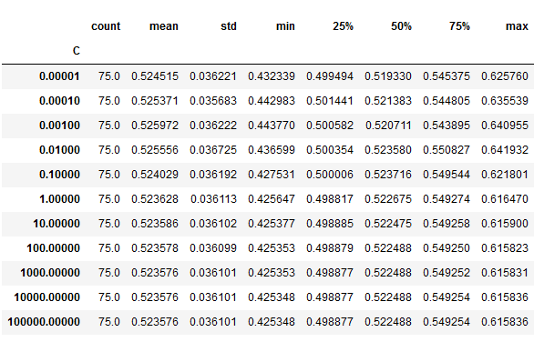
結果のプロット
def plot_ic_distribution(df, ax=None):
if ax is not None:
sns.distplot(df.ic, ax=ax)
else:
ax = sns.distplot(df.ic)
mean, median = df.ic.mean(), df.ic.median()
ax.axvline(0, lw=1, ls='--', c='k')
ax.text(x=.05, y=.9, s=f'Mean: {mean:8.2f}\nMedian: {median:5.2f}',
horizontalalignment='left',
verticalalignment='center',
transform=ax.transAxes)
ax.set_xlabel('Information Coefficient')
sns.despine()
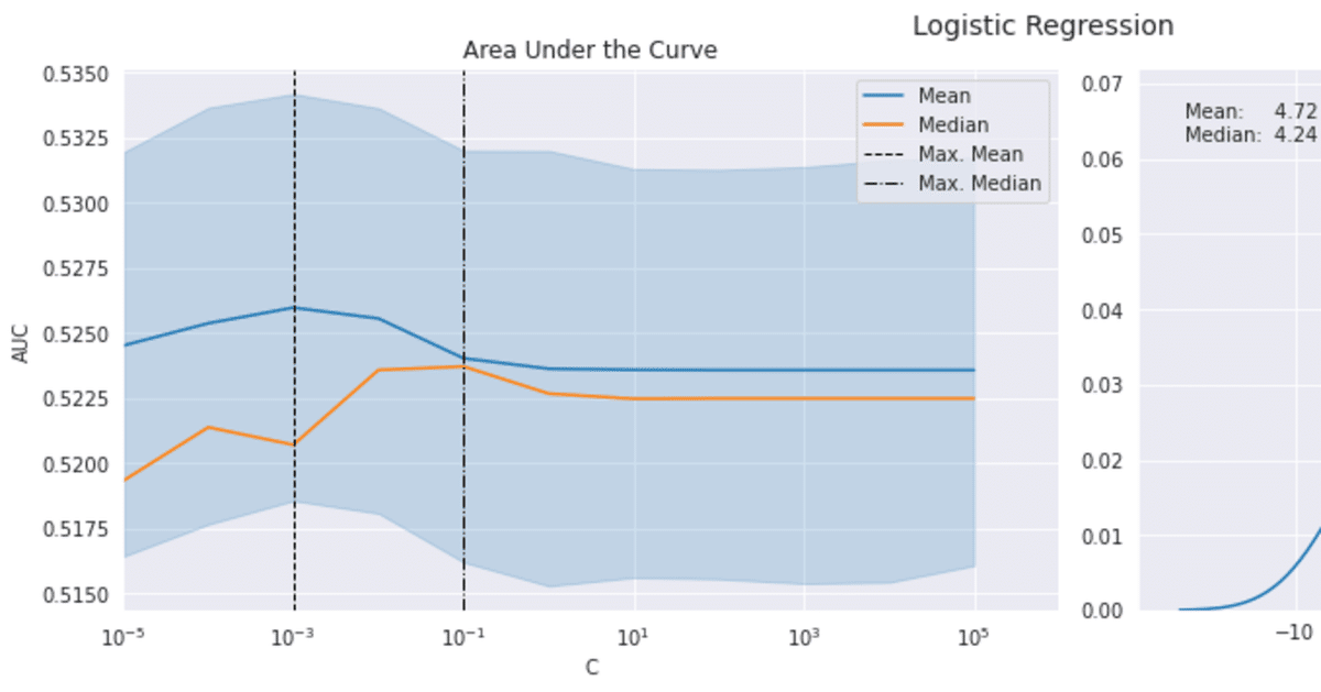
plt.tight_layout()fig, axes= plt.subplots(ncols=2, figsize=(15, 5))
sns.lineplot(x='C', y='auc', data=log_scores, estimator=np.mean, label='Mean', ax=axes[0])
by_alpha = log_scores.groupby('C').auc.agg(['mean', 'median'])
best_auc = by_alpha['mean'].idxmax()
by_alpha['median'].plot(logx=True, ax=axes[0], label='Median', xlim=(10e-6, 10e5))
axes[0].axvline(best_auc, ls='--', c='k', lw=1, label='Max. Mean')
axes[0].axvline(by_alpha['median'].idxmax(), ls='-.', c='k', lw=1, label='Max. Median')
axes[0].legend()
axes[0].set_ylabel('AUC')
axes[0].set_xscale('log')
axes[0].set_title('Area Under the Curve')
plot_ic_distribution(log_scores[log_scores.C==best_auc], ax=axes[1])
axes[1].set_title('Information Coefficient')
fig.suptitle('Logistic Regression', fontsize=14)
sns.despine()
fig.tight_layout()
fig.subplots_adjust(top=.9);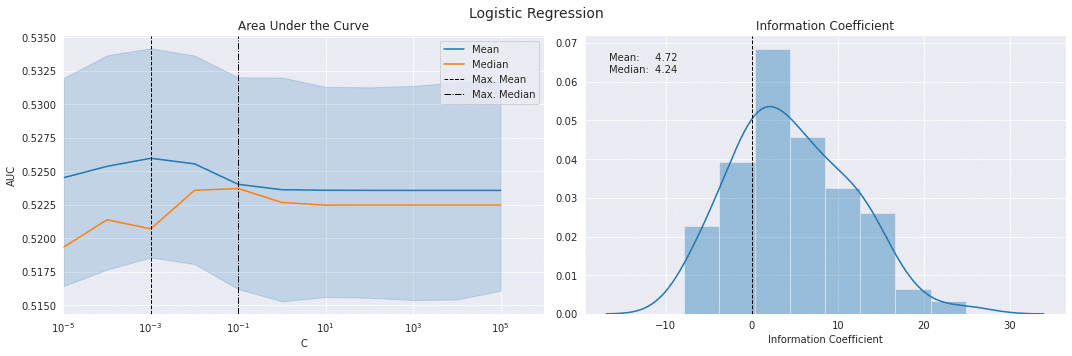
この記事が気に入ったらサポートをしてみませんか?