第7章 線形モデル編: 第6節 Alphalensを用いて分析する

はじめに
Alphalensとは?
Alphalensとは分析に特化したpythonライブラリです。今回は本ライブラリを用いて特徴量分析を行いたいと思います。モチベーションとしましては、前回の記事で予測値を出しましたが、観測値と予測値を分析するにあたって、ICを見るだけでは物足りないので、もっと細かく分析しようという話です。
alphalensのgithubはこちらをご参照ください。
インポートと設定
import warnings
warnings.filterwarnings('ignore')
from pathlib import Path
import pandas as pd
from alphalens.tears import create_summary_tear_sheet
from alphalens.utils import get_clean_factor_and_forward_returnsidx = pd.IndexSliceデータの読み込み
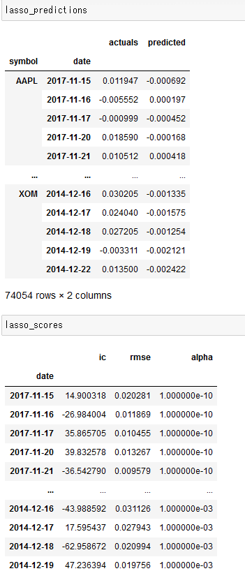
こちらでは前回の記事で第7章 線形モデル編: 第5節 線形回帰で株価予測をするで行った3つのモデルの出力結果を読み込みます。データセットのフォーマットとしてはscoresは残差や情報係数、アルファの情報が入っていて、predictionsが観測値と予測値である。
with pd.HDFStore('data.h5') as store:
   lr_predictions = store['lr/predictions']
   lasso_predictions = store['lasso/predictions']
   lasso_scores = store['lasso/scores']
   ridge_predictions = store['ridge/predictions']
   ridge_scores = store['ridge/scores']
DATA_STORE = Path('..', 'data', 'assets.h5')def get_trade_prices(tickers, start, stop):
prices = (pd.read_hdf(DATA_STORE, 'quandl/wiki/prices').swaplevel().sort_index())
prices.index.names = ['symbol', 'date']
prices = prices.loc[idx[tickers, str(start):str(stop)], 'adj_open']
return (prices
.unstack('symbol')
.sort_index()
.shift(-1)
.tz_localize('UTC'))def get_best_alpha(scores):
return scores.groupby('alpha').ic.mean().idxmax()def get_factor(predictions):
return (predictions.unstack('symbol')
.dropna(how='all')
.stack()
.tz_localize('UTC', level='date')
.sort_index()) 線形回帰
lr_factor = get_factor(lr_predictions.predicted.swaplevel())
lr_factor.head()
'''
date                       symbol
2014-12-09 00:00:00+00:00  AAL       0.001839
                          AAPL     -0.001534
                          ABBV      0.001316
                          AGN       0.002175
                          AIG      -0.000336
dtype: float64
'''
tickers = lr_factor.index.get_level_values('symbol').unique()trade_prices = get_trade_prices(tickers, 2014, 2017)
trade_prices.info()
'''
<class 'pandas.core.frame.DataFrame'>
DatetimeIndex: 1007 entries, 2014-01-02 00:00:00+00:00 to 2017-12-29 00:00:00+00:00
Columns: 257 entries, AAL to YUM
dtypes: float64(257)
memory usage: 2.0 MB
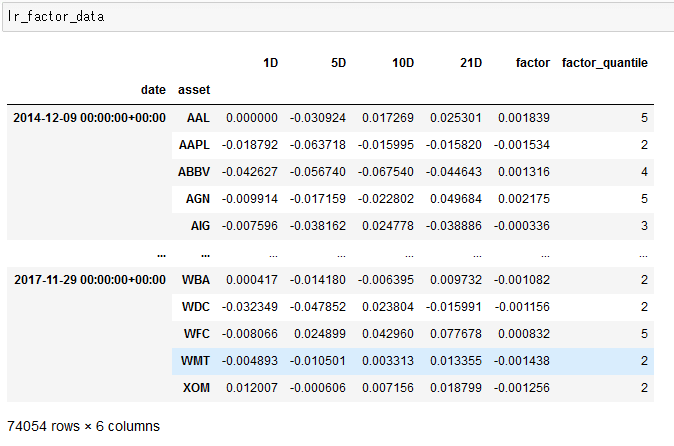
'''lr_factor_data = get_clean_factor_and_forward_returns(factor=lr_factor,
prices=trade_prices,
quantiles=5,
periods=(1, 5, 10, 21))
lr_factor_data.info()
'''
Dropped 0.0% entries from factor data: 0.0% in forward returns computation and 0.0% in binning phase (set max_loss=0 to see potentially suppressed Exceptions).
max_loss is 35.0%, not exceeded: OK!
<class 'pandas.core.frame.DataFrame'>
MultiIndex: 74054 entries, (Timestamp('2014-12-09 00:00:00+0000', tz='UTC'), 'AAL') to (Timestamp('2017-11-29 00:00:00+0000', tz='UTC'), 'XOM')
Data columns (total 6 columns):
# Column Non-Null Count Dtype
--- ------ -------------- -----
0 1D 74054 non-null float64
1 5D 74054 non-null float64
2 10D 74054 non-null float64
3 21D 74054 non-null float64
4 factor 74054 non-null float64
5 factor_quantile 74054 non-null int64
dtypes: float64(5), int64(1)
memory usage: 3.7+ MB
'''ここでget_clean_factor_and_forward_returnsは日次データから複数のフォワードリターン(periods指定)と分位数を指定する。分位数は、ファクターをランキング付けたもので、今回は5段階評価している。最小値から最大値までを均等に5分割して、ファクターがどの階級に入っているのかを表している。これからそこも含めて詳しく分析する。
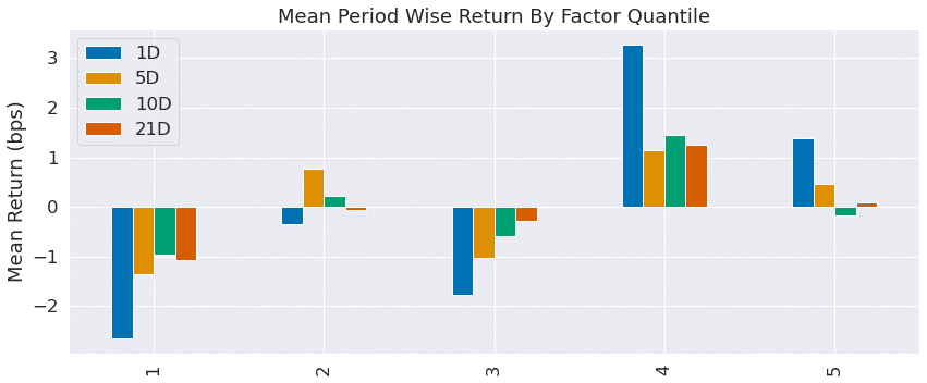
create_summary_tear_sheet(lr_factor_data);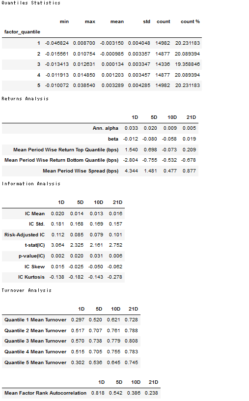
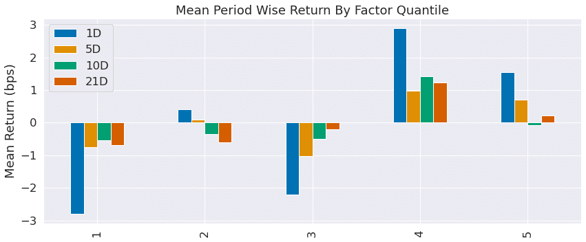
これらの表と図がalphalens.tears.create_summary_tear_sheetで一気に呼べるんですね。残り2つの回帰に関しても同じことをやるので、解説は割愛します。
リッジ回帰
best_ridge_alpha = get_best_alpha(ridge_scores)
ridge_predictions = ridge_predictions[ridge_predictions.alpha==best_ridge_alpha].drop('alpha', axis=1)
ridge_factor = get_factor(ridge_predictions.predicted.swaplevel())ridge_factor_data = get_clean_factor_and_forward_returns(factor=ridge_factor,
prices=trade_prices,
quantiles=5,
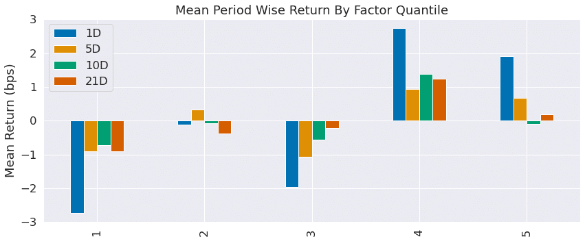
periods=(1, 5, 10, 21))create_summary_tear_sheet(ridge_factor_data);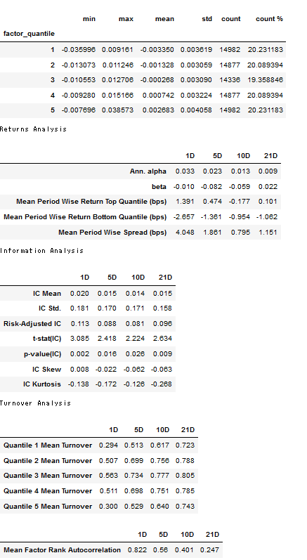
ラッソ回帰
best_lasso_alpha = get_best_alpha(lasso_scores)
lasso_predictions = lasso_predictions[lasso_predictions.alpha==best_lasso_alpha].drop('alpha', axis=1)
lasso_factor = get_factor(lasso_predictions.predicted.swaplevel())lasso_factor_data = get_clean_factor_and_forward_returns(factor=lasso_factor,
prices=trade_prices,
quantiles=5,
periods=(1, 5, 10, 21))create_summary_tear_sheet(lasso_factor_data);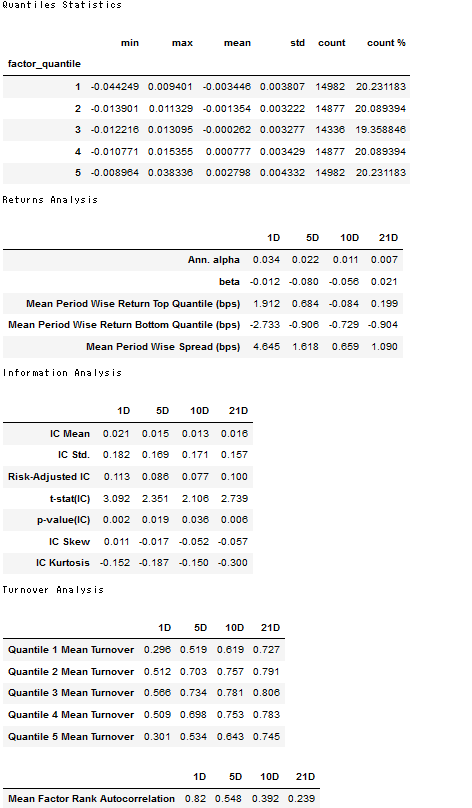
この記事が気に入ったらサポートをしてみませんか?