ファイナンス機械学習:交差検証によるハイパーパラメータの調整: Grid Search

時系列に跨った関数を扱う場合、情報のリーケージを防ぐために、テストデータと検証データを単純に切り分ける方法でなく、パージングを入れた切り分け方法を使用することが第一に重要である。
Grid Search CV
グリッドサーチは、ハイパーパラメータの全空間を網羅して逐次評価する方法である。データの基本構造が未知な場合に、最初に取るべき妥当な方法と言える。
scikit-learnに実装されているGrid SearchCVに、パージされたKfold Classを渡すコードがスニペット9.1に示されている。
def clfHyperFitGS(feat, lbl, t1, pipe_clf, param_grid, cv = 3,
                 bagging= [0, None, 1.], n_jobs= -1,
                 pctEmbargo= 0.0, **fit_params):
    import FinCV as fcv
    '''
        Returns:
            gs : fitted best estimator found by grid search
    '''
    if set(lbl.values) == {0, 1}:
        scoring='f1'    # f1 for meta-labeling
    else:
        scoring='neg_log_loss'    # symmetric towards all cases
    inner_cv = fcv.PurgedKFold(n_splits=cv, t1=t1, pctEmbargo=pctEmbargo)    # purged
    gs=GridSearchCV(estimator=pipe_clf ,param_grid=param_grid,
                    scoring=scoring, cv=inner_cv, n_jobs=n_jobs)
    gs = gs.fit(feat, lbl, **fit_params).best_estimator_    # pipeline
    if bagging[1] is not None and bagging[1] > 0:
        gs = BaggingClassifier(base_estimator=MyPipeline(gs.steps),
                               n_estimators=int(bagging[0]),
                               max_samples=float(bagging[1]),
                               max_features=float(bagging[2]), n_jobs=n_jobs)
        gs = gs.fit(feat, lbl, sample_weight=fit_params[gs.base_estimator.steps[-1][0]+'__sample_weight'])
        gs = Pipeline([('bag', gs)])
    return gs
MyPipeline
sklearnのPipelineでは、sample_weightの引数渡しは、**fit_paramsで渡さなければならないので、改良するために、Pipelineクラス拡張してsample_weightを渡せるようにしたのが、スニペット9.2である。
from sklearn.pipeline import Pipeline
class MyPipeline(Pipeline):
    def fit(
        self, X, y, sample_weight = None, **fit_params) :
        if sample_weight is not None:
            fit_params[self.steps[-1][0] + '__sample_weight'] = sample_weight
        return super(MyPipeline,self).fit(X, y, **fit_params)
RandomizedSearchCV
サーチするパラメータの数が多い場合、GridSearchでは計算負荷が大きくなる。よって、分布からパラメータをサンプリングすることで、負荷を下げるRandomizedSearchCVを使用できるように、上記のclfHyperFitGSを拡張する。
def clfHyperFit(feat, lbl, t1, pipe_clf, param_grid, cv = 3,
                 bagging= [0, None, 1.], rndSearchIter=0, n_jobs= -1,
                 pctEmbargo= 0.0, **fit_params):
  import FinCV as fcv

    '''
            rndSearchIter (int): number of iterations to use in randomized GS (if 0 then apply standard GS)

        Returns:
            gs: fitted best estimator found by grid search
    '''
    if set(lbl.values) == {0, 1}:
        scoring='f1'    # f1 for meta-labeling
    else:
        scoring='neg_log_loss'    # symmetric towards all cases
    inner_cv = fcv.PurgedKFold(n_splits=cv, t1=t1, pctEmbargo=pctEmbargo)    # purged

    if rndSearchIter == 0:

        gs = GridSearchCV(estimator=pipe_clf, param_grid=param_grid,
                          scoring=scoring, cv=inner_cv, n_jobs=n_jobs)
    else:
        gs = RandomizedSearchCV(estimator=pipe_clf, param_distributions=param_grid,
                                scoring=scoring,
                                cv=inner_cv, n_jobs=n_jobs, n_iter=rndSearchIter)
    gs = gs.fit(feat, lbl, **fit_params).best_estimator_    # pipeline

    if bagging[1] is not None and bagging[1] > 0:
        gs = BaggingClassifier(estimator=MyPipeline(gs.steps),
                               n_estimators=int(bagging[0]),
                               max_samples=float(bagging[1]),
                               max_features=float(bagging[2]), n_jobs=n_jobs)
        gs = gs.fit(feat, lbl, sample_weight=fit_params[gs.base_estimator.steps[-1][0]+'__sample_weight'])
        gs = Pipeline([('bag', gs)])
    return gs
対数一様分布
グリッドサーチやランダムサーチで探査するパラメータの値は負ではないが、その値域は広い。またその値に一様に線形応答するとは限らず、$${[0,100]}$$領域の一様分布からあるパラメータをサンプリングすることは非効率である。よってそれらの対数が一様に分布する分布から値を生成する方法の方が効率が良い。
確率変数$${x}$$が、正の数の$${a}$$を使い、$${x \sim U[a,b]}$$で分布しているとする。これは、$${\log x \sim U[\log a, \log b]}$$に等しい。
対数の一様分布のCDF(累積分布関数)は、
$${F(x)=\displaystyle{\left\{ \begin{array}{ll} \frac{\log x - \log a}{\log b - \log a} & (a \geq x \geq b) \\ 0 & (x < a) \\ 1 & (x>b) \end{array} \right.}}$$
となり、これを微分して、確率密度関数は、
$${f(x)=\displaystyle{\left\{ \begin{array}{ll} \frac{1}{x\log (\frac{b}{a})} & (a \geq x \geq b) \\ 0 & (x < a) \\ 0 & (x>b) \end{array} \right.}}$$
と与えられる。
この関数は、対数の底に対して不変である。
対数一様分布はscipy.statsにloguniformとして実装されている。これを使って、スニペット9.4と同様にコルモゴロフ–スミルノフ検定を行ってみる。
from scipy.stats import loguniform
a, b, size = 1e-3, 1e3, 10000
vals = loguniform.rvs(a = a, b= b,size=size)
print(kstest(rvs=np.log(vals), cdf='uniform', args=(np.log(a), np.log(b / a)), N=size))
print(pd.Series(vals).describe())
plt.figure(figsize=(11, 5))
plt.subplot(121)
pd.Series(np.log(vals)).hist()
plt.subplot(122)
pd.Series(vals).hist()
plt.show()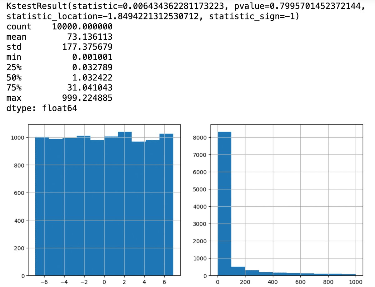
p値は0.05以上で、正規分布を満たしている。
scoring
上記のスニペットには、ラベル適用モデルに対して、ハイパーパラメター探索のスコアリングにf1が指定され、ラベル以外ではneg_log_lossを指定している。
投資戦略のためにハイパーパラメータを調整するときは、正確率ではなくneg_log_lossを使用した方が良い。なぜなら、neg_log_lossは予測の確信度を考慮に入れてスコアリングするからで、もしも単純に正確さとするならば、2回の予測に[1,1]と出し、正解が[1,0]だった場合、正解率は0.5である。
これを同様に、neg_log_lossで評価すると、以下のグラフになる。
def NegLogLoss(y_pred,pred_proba,eps=1e-15):
    pred_proba=np.clip(pred_proba,eps,1-eps)
    score=1.0
    n_samples=len(y_pred)
    for i in range(n_samples):
        score*=pred_proba[i,y_pred[i]]
    return -np.log(score)/float(n_samples)

p=list(np.linspace(0.5,0.9,50))
p=np.round(p,2)
LogLoss = pd.DataFrame(index=p,columns=p, dtype=float)

y_pred=np.array([1,1])

for x in p:
    ll=[]
    for y in p:
        pred_proba=np.array([[x,1-x],[1-y,y]])
        ll.append(NegLogLoss(y_pred,pred_proba))
    LogLoss.loc[x]=ll

labels = np.linspace(0.5, 0.9, 10)
labels = np.round(labels,2)

ticks = []
for label in labels:
    idx_pos = LogLoss.index.get_loc(label)
    ticks.append(idx_pos)

fig, ax = plt.subplots(figsize=(7, 7))
cLogLoss = ax.matshow(LogLoss,origin='lower',interpolation='nearest')
ax.set_yticks(ticks)
ax.set_yticklabels(labels)
ax.set_xticks(ticks)
ax.set_xticklabels(labels)
ax.set_xlabel('prob for the 1st for 1')
ax.set_ylabel('prob for the 2nd for 0')
ax.tick_params(axis="x", bottom=True,labelbottom=True,labeltop=False)

fig.colorbar(cLogLoss)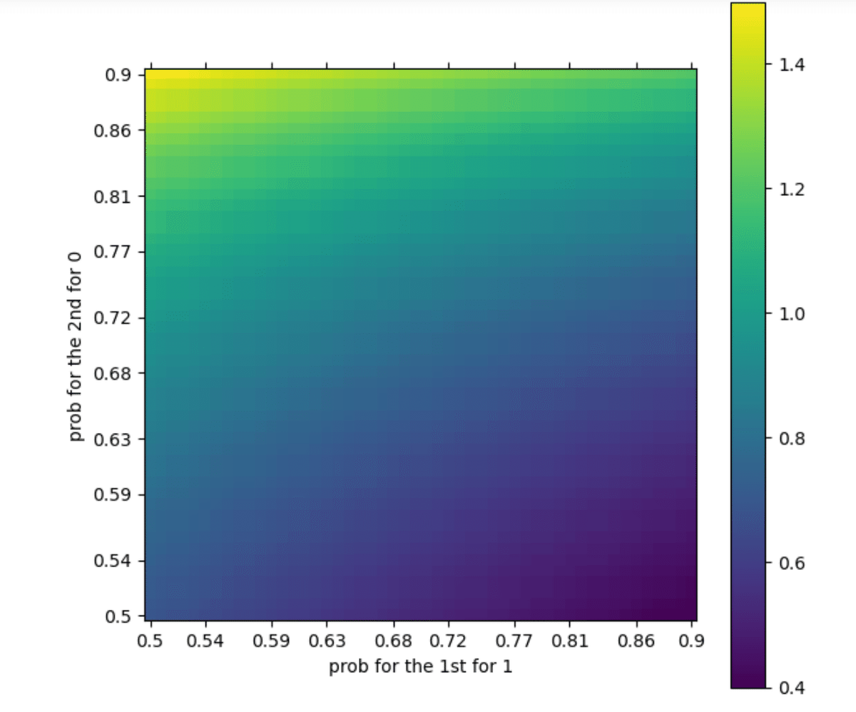
最初は1と予想されて1と出し、2回目は、0の予想にも関わらず1を出した場合、ゼロの予想確率(確信)が高い時に1を出した時の方がペナルティは高く評価される。
投資戦略はある証券を高く確率で買うべきだと予測し、その確信度に応じてベットサイズを決定し、ロングポジションを取る。予測が間違っている時には、市場で価格が暴落し損失を出す。
正解率は、確率の高い誤購入と確率の低い誤購入を同等に扱うが、投資戦略では適切なラベルを高い確信度で予測することが利益を生むことにつながるため、確信度を考慮に入れなければならない。よって、評価にも確信度を入れるneg_log_lossが最適なのである。