Mapleで制御工学の基礎虎の巻10「最適制御」

前々回の記事では固有値を配置することでシステムの応答を調整できることを紹介しました。そして前回の記事では固有値の変え方によって応答が変わることも紹介しました。今回は評価関数を最適にする固有値になるような状態フィードバックゲインKを求める方法を紹介します。固有値を直接設定するのではなく、評価関数を最適にするKをリカッチ方程式を解くことで求めます。結果的に設定した評価関数が最適になる固有値を持つシステムになるわけです。
なお評価関数は目的に応じて作ることができますが、一般的な評価関数は状態と入力の２次形式を用います。本記事でも最も基本的なこの形の評価関数を用いることにします。評価関数を一応載せておきますが、あまり気にする必要はありません。QとRだけ気にしておけば十分です。Qは状態xの次数の正方行列で、Rは入力uの次数の正方行列になります。xが２次ならQは２次の正方行列、uが１次、要するに単入力の場合スカラーになります。QとRを変えるとどのように影響するかは後半で紹介します。

評価関数

対象システム

本記事で最適制御を試みるシステムを以下に示します。
１入力の２次のシステムです。最適制御は出力は関係ないのでC行列やD行列については本記事では設定していません。

システムの状態空間表現

プログラム

リカッチ方程式を解く「CARE」コマンドを使うために「DynamicSystems」ライブラリを呼び出します。また各種の行列演算を行うために「LinearAlgebra」ライブラリを呼び出します。
先のシステムの状態空間表現を定義し、重みQとrを設定します。あとは「CARE」コマンドでリカッチ方程式を解きます。リカッチ方程式の解Pを用いてフィードバック行列Kを求めるだけです。
これで評価関数を最小にするフィードバックゲインKを求めることができるのです。

# 最適制御　Optimal control
restart;
with(DynamicSystems);
with(LinearAlgebra);

# 状態空間モデル　State space model　
A := Matrix([[0, 1], [-1, -0.2]])
B := Matrix([[0], [1]]);

# 重み行列　Weighting matrix
Q := Matrix([[10, 0], [0, 1]]);
r := Matrix([1]);

# リカッチ代数方程式の解P　Solution of Riccati's algebraic equation P
P := CARE(A, B, Q, r);

# 最適制御の状態フィードバックゲインK　Optimal control state feedback gain K
K := ((MatrixInverse(r)) . (Transpose(B))) . P;

システムの応答

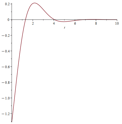
設定したQとrの重みに対応するシステム応答、図１にインパルス応答を与えたときの状態の応答を、図２に状態フィードバックの入力の応答を示します。これだけだと「最適なんですね」と納得するしかありませんので、重みを変えたときの応答の変化を見てみましょう。

図１　インパルス入力を与えた時の状態の応答

図２　状態フィードバック入力のインパルス応答

重みrを変更してみる

入力の重みｒを「１」から「２」に大きくしてみます。
図４の入力が少し小さくなっている（先ほどより制限されている）のがわかりますね。一方で図３のx1の応答が大きくなっているのがわかります。インパルス外乱を抑制する入力が小さくなったため、x１の抑制力が減っているためです。
入力の重みrを大きくすると相対的に入力が制限されることがわかります。一方で状態の抑制力が減ってしまいます。入力と状態の応答を見ながらハイパーパラメータである重みrを調整するとよいです。

図３　インパルス入力を与えた時の状態の応答（rを変更）

図４　状態フィードバック入力のインパルス応答（rを変更）

重みQを変更を変更してみる

次に状態の重みQを変えてみましょう。重み行列Qの１行１列の数値を10から5に小さくしてみます。
図５を見ると変更前の図３に比べてx1の応答は大きくなってしまっているのがわかります。重みを小さくすると対応する状態の変化が大きくなるのです。その分、相対的に入力を小さくなっていることが図６を見るとわかります。
今回の例ではx1に対応する重み行列Qの１行１列の数値を変えたことによりx2の応答に目に見える大きな影響が見られませんでしたが、x1に対応する重み部分とx2に対応する重み行列の部分の相対的な大きさの違いにより、影響を受けることがあります。今回のシステムの場合、入力、x1、x2の応答の影響を見ながら重みを適切に設定することが肝要です。

図５　インパルス入力を与えた時の状態の応答（Qを変更）

図６　状態フィードバック入力のインパルス応答（Qを変更）

最適制御は評価関数を最適にする状態フィードバック行列Kを求める手法ですが、入力の重み、状態の重みという２つのパラメータによって調整する手法を読み替えることができます。要するに重み行列Qとrというハイパーパラメータによるシステムの特性設定ができるようにしたとも言えます。

【English】

In the previous article, I showed how the response of a system can be adjusted by placing eigenvalues. And in another previous article, I also showed how the response can be changed by modifying the eigenvalues. In this article, I will show you how to find the state feedback gain K such that the eigenvalues are the optimal ones for the evaluation function. Instead of setting the eigenvalues directly, K that optimizes the evaluation function is obtained by solving the Riccati equation. The result is a system with eigenvalues that make the set evaluation function optimal.
Although evaluation functions can be created for any purpose, general evaluation functions use a quadratic form of state and input. This article also uses the most basic evaluation function of this form. Q is a square matrix of the order of the state x, and R is a square matrix of the order of the input u. If x is quadratic, Q is a square matrix of the second order, and if u is first order, in essence, a scalar. We will show how changing Q and R affects the results later in this section.

Evaluation function

Target system

The system for which optimal control is attempted in this article is shown below; it is a one-input, second-order system. Since the output is irrelevant for optimal control, the C and D matrices are not set in this article.

State Space Representation of the System

Program

Calls the “DynamicSystems” library to use the “CARE” command to solve Riccati equations. It also calls the “LinearAlgebra” library to perform various matrix operations.
Define the state-space representation of the previous system and set the weights Q and r. Now solve the Riccati equation with the “CARE” command. Simply use the solution P of the Riccati equation to find the feedback matrix K. We can now find the feedback gain K that minimizes the evaluation function.

# Optimal control
restart;
with(DynamicSystems);
with(LinearAlgebra);

# State space model　
A := Matrix([[0, 1], [-1, -0.2]])
B := Matrix([[0], [1]]);

# Weighting matrix
Q := Matrix([[10, 0], [0, 1]]);
r := Matrix([1]);

# Solution of Riccati's algebraic equation P
P := CARE(A, B, Q, r);

# Optimal control state feedback gain K
K := ((MatrixInverse(r)) . (Transpose(B))) . P;

System Response

The system response corresponding to the set Q and r weights, Figure 1 shows the response of the state when given an impulse response, and Figure 2 shows the response of the state feedback input. With just this, we can only agree that it is optimal, so let's see how the response changes when the weights are changed.

Figure 1. State response when impulse input is given

Figure 2. Impulse response of state feedback input

Try changing the weight r

Let's increase the input weight r from “1” to “2”. You can see that the input in Figure 4 has become a little smaller (more restricted than before). On the other hand, you can see that the response of x1 in Figure 3 has become larger. This is because the input that suppresses the impulse disturbance has become smaller, so the suppression of x1 has decreased.
It can be seen that increasing the input weight r causes the input to be relatively more restricted. On the other hand, the inhibiting power of the state decreases. It is best to adjust the weight r, the hyperparameter, by watching the response of the input and the state.

Figure 3. State response when impulse input is given (when r is changed)

Figure 4. Impulse response of state feedback input (when r is changed)

Try changing the weight Q

Next, let's change the state weights Q. Let's decrease the number of rows and columns in the weight matrix Q from 10 to 5. Figure 5 shows that the response of x1 has become larger than in Figure 3 before the change. When we reduce the weights, the corresponding state change becomes larger. Figure 6 shows that the input has become relatively smaller.
In this example, changing the numerical values of one row and one column of the weight matrix Q corresponding to x1 had no visible significant effect on the response of x2, but it can be affected by the difference in relative size of the weight portion corresponding to x1 and the weight matrix portion corresponding to x2. In the case of this system, it is essential to set the weights appropriately while watching the impact of the input, x1, and x2 responses.

Figure 5. State response when impulse input is given (when Q is changed)

Figure 6. Impulse response of state feedback input (when Q is changed)

Optimal control is a method of finding the state feedback matrix K that optimizes the evaluation function, but it can be read as a method of adjusting by two parameters: input weights and state weights. In essence, it can be said that the hyperparameters of the weight matrices Q and r allow for setting the characteristics of the system.

【Sample】

Created by Maple 2024.1

Demo_OptControl_3.mw

111 KB

ファイルダウンロードについて

ダウンロード