Mapleで制御工学の基礎虎の巻12「カルマンフィルタ」

齋藤芳明

2025年1月25日 23:12

前回の記事ではオブザーバについて紹介を行いましたが、状態を推定する方法としてカルマンフィルタがあります。今回はカルマンフィルタを使って状態を推定する方法について紹介します。

カルマンフィルタは、動的システムの状態を観測データからリアルタイムで推定するアルゴリズムです。ノイズの影響を受けた測定値やシステムモデルが不完全でも、推定を最適化できる特徴があります。

基本的な流れ

予測ステップ

・現在の状態とモデルから次の状態を予測
・状態推定値と誤差共分散を更新

更新ステップ

・新しい観測値を使って予測を修正
・カルマンゲインを計算して、観測と予測のバランスを調整

Mapleでカルマンフィルタを作ってみよう！

実際にMaple を使ってカルマンフィルタの計算手順を見てみると理解しやすいと思うので、順を追って説明していきたいと思います。

行列やベクトルを扱うため「LinearAlgebra」のライブラリを読み込みます。また、確率的な誤差を持つデータの推定を行うため乱数を発生させます。そのため、乱数を発生させる関数を呼ぶための「Statistics」ライブラリを読み込みます。

with(LinearAlgebra); # 行列やベクトルを扱うために必要
with(Statistics); # 乱数を発生させるのに必要

次に状態を推定する対象のシステムを設定します。

# パラメータの設定
dt := 1;  # 時間ステップ
A := Matrix([[1, dt], [0, 1]]);  # 状態遷移行列
B := Vector([0, 0]);  # 制御入力行列（今回は使用しない）
H := Vector[row]([1, 0]);  # 観測行列

システムに影響するプロセスノイズと観測値に影響する観測ノイズを定義します。要するにどのくらいのノイズが生じるかはわかっているというのが前提となります。とは言え、ある程度わかっていれば大丈夫です。

Q := Matrix([[0.1, 0], [0, 0.1]]);  # プロセスノイズ共分散行列
R := 0.1;  # 観測ノイズ共分散（スカラー値）

状態と誤差共分散行列の初期値を設定します。

# 初期状態の設定
x := Vector([0, 1]);  # 状態ベクトルの初期値 [位置, 速度]
P := Matrix([[1, 0], [0, 1]]);  # 誤差共分散行列の初期値

次に時系列データを準備します。
今回は50ステップ分のデータを用意して状態を推定することにします。

# データ生成の準備
N := 50;  # データポイント数
true_state := Matrix(2, N);  # 真の状態を保存する行列
observations := Vector(N);  # 観測値を保存するベクトル

ノイズを与えるため、今回は正規分布に従う乱数を使うことにします。

# 正規分布に従う乱数生成の準備
X := RandomVariable(Normal(0, 1));

真の状態にもシステムノイズを与え、観測値にも観測ノイズを与えます。

# 真の状態と観測値の生成
for k to N do
    true_state[1, k] := k*dt + 0.1*Sample(X, 1)[1];  # 真の位置（ノイズを含む）
    true_state[2, k] := 1 + 0.1*Sample(X, 1)[1];  # 真の速度（ノイズを含む）
    observations[k] := true_state[1, k] + sqrt(R)*Sample(X, 1)[1];  # 観測値（位置 + 観測ノイズ）
end do;

そして、いよいよカルマンフィルタ部分になります。
以下のプログラムを見るとわかりますが、予測ステップと更新ステップを繰り返しているだけです。
予測ステップでは１つ前の状態から次の状態を求めるのと、誤差共分散行列の予測をします。
更新ステップではまずカルマンゲインを計算し、そのカルマンゲインから状態を更新します。同じく誤差共分散行列の更新をするだけです。
あとは推定した状態を保存しているだけのシンプルなプログラムになります。

# カルマンフィルタの実装
estimated_state := Matrix(2, N);  # 推定された状態を保存する行列

for k to N do
    # 予測ステップ
    x := (A . x) + B*0;  # 状態の予測（制御入力はゼロ）
    P := ((A . P) . (Transpose(A))) + Q;  # 誤差共分散行列の予測

    # 更新ステップ
    K := P . (Transpose(H))/(((H . P) . (Transpose(H))) + R);  # カルマンゲインの計算
    x := x + K*(observations[k] - (H . x));  # 状態の更新
    P := (Matrix([[1, 0], [0, 1]]) - (K . H)) . P;  # 誤差共分散行列の更新

    # 推定された状態の保存
    estimated_state[1, k] := x[1];  # 推定位置
    estimated_state[2, k] := x[2];  # 推定速度
end do;

それでは推定した位置を見てみましょう。
真の位置、それを誤差を含んだ観測値も合わせて図１に示しています。
位置は観測しているので推定値は大きくは外れていませんね。

# プロット（位置）
plots[display]([plots[pointplot]([seq([k*dt, observations[k]], k = 1 .. N)], color = red, symbol = solidcircle), plots[pointplot]([seq([k*dt, true_state[1, k]], k = 1 .. N)], color = green), plots[pointplot]([seq([k*dt, estimated_state[1, k]], k = 1 .. N)], color = blue)], title = "Kalman Filter for 2nd Order System", legend = ["Observations", "True Position", "Estimated Position"], labels = ["Time step", "Position"]);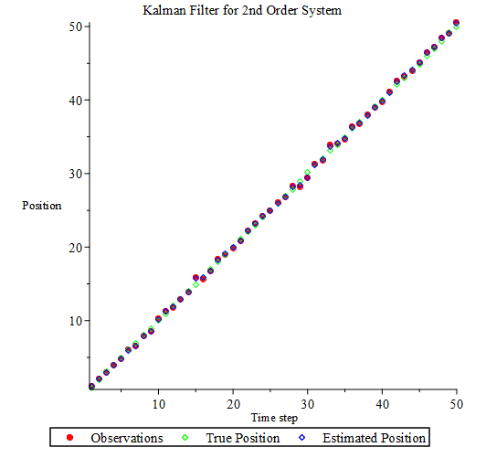

観測していない状態である速度の方を見てみましょう。
図２には真の速度、推定した速度、推定値と真の値との差を示しています。
この差をどう判断するかは設計者の判断によりますが、差異を許容できなければパラメータ調整するか、モデル自体を改善していく必要があります。

# プロット（速度）
plots[display]([plots[pointplot]([seq([k*dt, true_state[2, k]], k = 1 .. N)], color = green), plots[pointplot]([seq([k*dt, estimated_state[2, k]], k = 1 .. N)], color = blue), plots[pointplot]([seq([k*dt, estimated_state[2, k] - true_state[2, k]], k = 1 .. N)], style = line, color = red)], title = "Kalman Filter for 2nd Order System", legend = ["True Speed", "Estimated Speed", "Estimated-True"], labels = ["Time", "Speed"])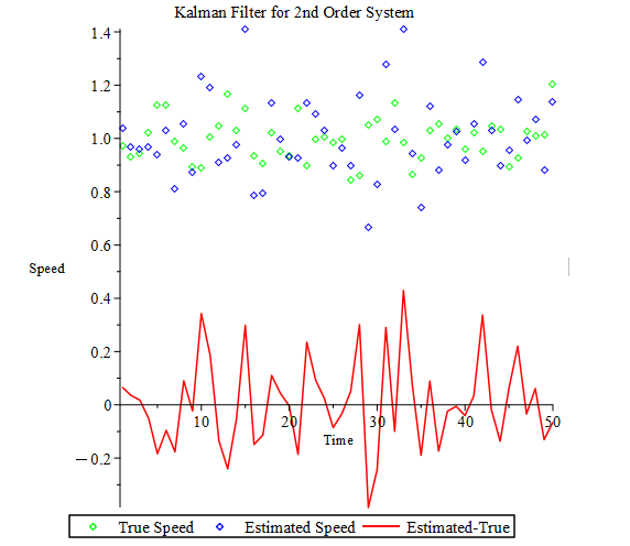

いかがでしょうか？
カルマンフィルタ自体はそんなに難しいものではないと思われたのではないでしょうか？
ノイズを含んだシステムの状態を推定する場合にはカルマンフィルタを使うとある程度状態を推定することができます。基本のカルマンフィルタでは対象とするシステムは線型システムを前提としていますが、非線形なシステムにも使える拡張カルマンフィルタという手法もあります。
次の記事では拡張カルマンフィルタについて見ていきたいと思います。

【English】

In the previous article, I introduced Observer, and the Kalman filter is a method for estimating states. In this article, I will introduce how to use the Kalman filter to estimate the states.

The Kalman filter is an algorithm that estimates the states of a dynamic system in real time from observed data. It has the feature of being able to optimize the estimation even when measurements are affected by noise or the system model is incomplete.

Basic Flow

Prediction Step

・Predicts the next states from the current states and model
・Update states estimate and error covariance

Update step

・Revise predictions using new observations
・Calculate Kalman gain to balance observations and forecasts

Let's create Kalman Filter in Maple!

It will be easier to understand if you actually look at the procedure for calculating the Kalman filter using Maple, so I will explain it step by step.

It loads the “LinearAlgebra” library to use matrix and vector functions. We will also use random numbers to estimate data with stochastic errors. Therefore, we load the “Statistics” library to use functions that generate random numbers.

with(LinearAlgebra); # For matrices and vectors
with(Statistics); # For generating random numbers

Next, set up the target system whose states are to be estimated.

# Parameter settings
dt := 1;  # Time Step
A := Matrix([[1, dt], [0, 1]]);  # State transition matrix
B := Vector([0, 0]);  # Control input matrix (not used this time)
H := Vector[row]([1, 0]);  # Observation matrix

We define the process noise that affects the system and the observed noise that affects the observed values. In essence, it is assumed that we know how much noise will be caused. However, it is only okay if you know some of it.

Q := Matrix([[0.1, 0], [0, 0.1]]);  # Process noise covariance matrix
R := 0.1;  # Observation noise covariance (scalar value)

Sets initial values for the states and the error covariance matrix.

# Initial state setting
x := Vector([0, 1]);  # Initial value of state vector [position, velocity]
P := Matrix([[1, 0], [0, 1]]);  # Initial values of the error covariance matrix

Next, prepare time series data. In this case, we will prepare data for 50 steps to estimate the states.

# Preparation for data generation
N := 50;  # Number of data points
true_state := Matrix(2, N);  # Matrix to record the true state
observations := Vector(N);  # Vector to record observations

To provide noise, we will use random numbers that follow a normal distribution.

# Preparation for random number generation following a normal distribution
X := RandomVariable(Normal(0, 1));

It also adds system noise to the true state and observation noise to the observed value.

# Generation of true states and observables
for k to N do
    true_state[1, k] := k*dt + 0.1*Sample(X, 1)[1];  # True position (including noise)
    true_state[2, k] := 1 + 0.1*Sample(X, 1)[1];  # True velocity (including noise)
    observations[k] := true_state[1, k] + sqrt(R)*Sample(X, 1)[1];  # Observed value (position + observed noise)
end do;

And now comes the Kalman filter part. As you can see in the following program, we just repeat the prediction step and the update step. In the prediction step, the next state is obtained from the previous state and the error covariance matrix is predicted.
The update step first computes the Kalman gain and then updates the states from that Kalman gain. The same just updates the error covariance matrix. The rest of the program is as simple as recording the estimated states.

# Kalman filter implementation
estimated_state := Matrix(2, N);  # Matrix to record the estimated states

for k to N do
    # Prediction Step
    x := (A . x) + B*0;  # Predicted states (zero control input)
    P := ((A . P) . (Transpose(A))) + Q;  # Predicting Error Covariance Matrices

    # Update Step
    K := P . (Transpose(H))/(((H . P) . (Transpose(H))) + R);  # Calculation of Kalman gain
    x := x + K*(observations[k] - (H . x));  # States Update
    P := (Matrix([[1, 0], [0, 1]]) - (K . H)) . P;  # Update error covariance matrix

    # Recording of presumed states
    estimated_state[1, k] := x[1];  # Estimated position
    estimated_state[2, k] := x[2];  # Estimated Speed
end do;

Now let's look at the estimated position. The true position, together with the observed position with errors, is shown in Figure 1. Since the position is observed, the estimated value is not far off.

# Plot (position)
plots[display]([plots[pointplot]([seq([k*dt, observations[k]], k = 1 .. N)], color = red, symbol = solidcircle), plots[pointplot]([seq([k*dt, true_state[1, k]], k = 1 .. N)], color = green), plots[pointplot]([seq([k*dt, estimated_state[1, k]], k = 1 .. N)], color = blue)], title = "Kalman Filter for 2nd Order System", legend = ["Observations", "True Position", "Estimated Position"], labels = ["Time step", "Position"]);

Figure 1. Estimation of state (position)

Let's look at the unobserved state, the velocity. Figure 2 shows the true velocity, the estimated velocity, and the difference between the estimated and true values. It is up to the designer to decide how to judge this difference, but if the difference is unacceptable, the parameters should be adjusted or the model itself should be improved.

# Plot (speed)
plots[display]([plots[pointplot]([seq([k*dt, true_state[2, k]], k = 1 .. N)], color = green), plots[pointplot]([seq([k*dt, estimated_state[2, k]], k = 1 .. N)], color = blue), plots[pointplot]([seq([k*dt, estimated_state[2, k] - true_state[2, k]], k = 1 .. N)], style = line, color = red)], title = "Kalman Filter for 2nd Order System", legend = ["True Speed", "Estimated Speed", "Estimated-True"], labels = ["Time", "Speed"])

You may have thought that the Kalman filter itself is not that difficult. When estimating the states of a system containing noise, the Kalman filter can be used to estimate the states to a certain extent. The basic Kalman filter assumes that the target system is a linear system, but there is also a method called the extended Kalman filter that can be used for nonlinear systems. In the next article, we will look at the extended Kalman filter.

【Sample】

Created by Maple 2024.1