
TimeGPT-1で時系列データの予測

TimeGPT-1とは?
TimeGPT-1は、トランスフォーマーベースのアーキテクチャで大量の多様な時系列データで事前に学習されたモデルとのことです。
文献[1]の実験では、ショートタームのパフォーマンスはLGBMが良いですが、ロングタームのパフォーマンスはTimeGPTが優れていたようです。

今回はこのTimeGPTを利用して時系列予測をしてみます。
まずはサイトにあるチュートリアルを動かしてみます。
実行環境はGoogle Corabです。
チュートリアル
インストール
pip install nixtlatsfrom nixtlats import TimeGPTtimegpt = TimeGPT(
token = '取得したAPIキーを設定する'
)下記サイトにログイン後に「Get Token」からAPIキーを取得し、APIキーを設定します。
timegpt.validate_token()こちらでTrueが出力されれば、正しくトークンの設定が出来ています。
時系列データの予測
import pandas as pd
df = pd.read_csv('https://raw.githubusercontent.com/Nixtla/transfer-learning-time-series/main/datasets/air_passengers.csv')
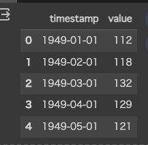
df.head()このチュートリアルでは、1949年から1960年までの月別の飛行機の乗客数データセットを使用しています。日付データは「timestamp」で表され、その月の乗客数は数値データとして「value」に格納されています。
timegpt.plot(df, time_col='timestamp', target_col='value')
それではtimegptのforecastで予測をしてみます。
指定するパラメーターは下記の通りです。
h : 予測のステップ数
freq : 時系列データの頻度をPandasのフォーマットで指定。MSは月間になります。
time_col : 日付のカラムを指定
target_col : 予測したいカラムを指定
timegpt_fcst_df = timegpt.forecast(df=df, h=12, freq='MS', time_col='timestamp', target_col='value')
timegpt_fcst_df.head()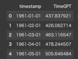
timegpt.plot(df, timegpt_fcst_df, time_col='timestamp', target_col='value')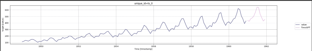
予測結果をプロットしてみます。
1960年1月からの予測がプロットされています。
ビットコインの価格を予測させてみる
次にビットコインの価格を予測させてみます。
pip install yfinanceyfinanceを利用してBTCJPYの価格データを取得します。
import yfinance

ticker = yfinance.Ticker("BTC-JPY")
df = ticker.history(period="max")
df.tail()
同じようにプロットしてみます。
timegpt.plot(df, time_col="Date", target_col='Close')
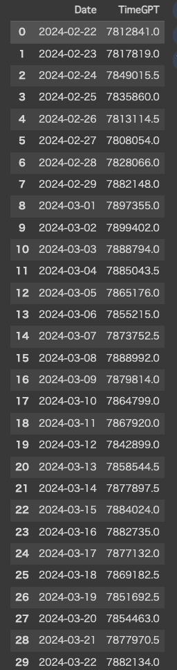
timegpt_fcst_df = timegpt.forecast(df=df, h=30, time_col='Date', target_col='Close', freq='D')30日分を予測してみました。
timegpt.plot(df, timegpt_fcst_df, time_col="Date", target_col='Close')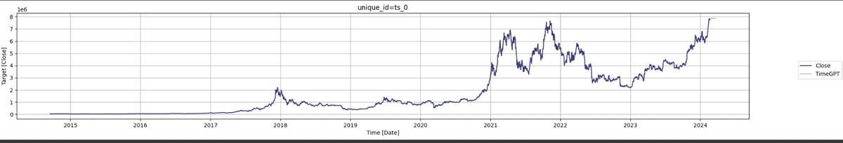
最後に予測分もプロットしてみます。
まとめ
今回は、TimeGPTを使って時系列データの予測を試しました。さらに、金融時系列データとしてビットコインの終値データも予測してみました。TimeGPTには、予測だけでなくアノマリー検知もできるようですので、次回はアノマリー検知も試してみたいと思います。
参考
[1] Azul Garza, Max Mergenthaler-Canseco. TimeGPT-1. arXiv. アクセス日 2024年2月21日, https://arxiv.org/abs/2310.03589