Autoencoderで異常検知

Autoencoderとは?
Autoencoderは、データの効率的な表現を学習するためのニューラルネットワークの一種です。特に、異常検知や次元削減、データのノイズ除去などに利用されます。
Autoencoderには、EncoderとDecoderがあります。
Encoder(エンコーダー):
入力データを圧縮して、低次元の潜在変数(潜在空間)にマッピングします。
これは、データの重要な特徴を抽出する役割を果たします。
Decoder(デコーダー):
潜在変数から元のデータに近いものを再構成します。
これは、圧縮された情報から元のデータを復元する役割を果たします。
Autoencoderは、入力データと再構成されたデータの間の誤差(再構成誤差)を最小化するように訓練されます。異常なデータに対しては再構成誤差が大きくなるため、この特性を利用して異常検知を行います。
この記事では、Autoencoderによる異常検知を行ってみます。
環境はGoogle Corabです。
データセットの用意
import pandas as pd
url = "https://raw.githubusercontent.com/Nixtla/transfer-learning-time-series/main/datasets/peyton_manning.csv"
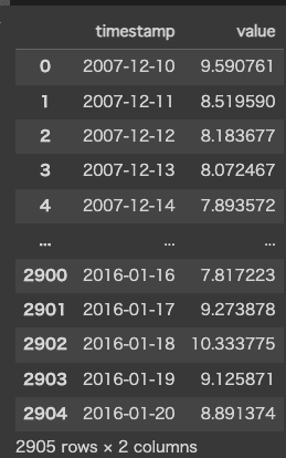
data = pd.read_csv(url)今回、異常検知に使用するデータセットはペイトン・マニングというアメフト選手のWikipediaアクセス数のデータです。日付データは「timestamp」で表され、アクセス数は数値データとして「value」に格納されています。
アクセス数のスケーリングを行っておきます。
from sklearn.preprocessing import MinMaxScaler

scaler = MinMaxScaler()
data['y'] = scaler.fit_transform(data[['value']])
Autoencoderモデルの構築
第1層から第3層までが、EncoderとDecoderの役割を果たしています。
Encoder部分で32次元まで圧縮した後に、Decoder部分で再び64次元に戻しています。
from keras import layers, models

input_dim = data[['y']].shape[1]

model = models.Sequential([
    layers.Dense(64, activation='relu', input_shape=(input_dim,)),
    layers.Dense(32, activation='relu'),
    layers.Dense(64, activation='relu'),
    layers.Dense(input_dim, activation='sigmoid')
])

model.compile(optimizer='adam', loss='mse')
モデルの訓練
train_size = int(len(data) * 0.8)
train_data = data['y'].values[:train_size]
test_data = data['y'].values[train_size:]

history = model.fit(train_data, train_data, epochs=50, batch_size=32, validation_split=0.1, shuffle=True)
異常検知の実施
再構成誤差の計算を行い、異常の検知を実施しています。
ここでは異常検知の閾値を95%として、検知を行っています。
import numpy as np

reconstructed_data = model.predict(test_data)
mse = np.mean(np.power(test_data - reconstructed_data, 2), axis=1)

threshold = np.percentile(mse, 95)

anomalies = mse > threshold
anomalies_indices = np.where(anomalies)[0]
異常の位置を可視化
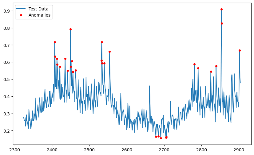
検知を行った異常の位置を可視化してみます。
import matplotlib.pyplot as plt

plt.figure(figsize=(10, 6))
plt.plot(data.index[train_size:], test_data, label='Test Data')
plt.plot(data.index[train_size:][anomalies_indices], test_data[anomalies_indices], 'ro', markersize=4, label='Anomalies')
plt.legend()
plt.show()
結果は下記の通りになりました。