
相手のショットスピード・ポジション別 合理的待機位置

こんにちは、トモヒトです。
今回は、相手のショットスピード・ポジション別に、合理的待機位置がどのように変化するかをみてみます。
前提条件
まずは、いくつかの前提条件をまとめておきます。
定数(物理定数、用具)
重力加速度=9.81m/s^2
空気密度=1.21kg/m^3
反発係数=0.75
摩擦係数=0.72
ボール半径=0.033m
ボールの質量=0.0577kg
変数
球速:90km/h~180km/hの範囲で5km/h刻み
ショットの打ち出し角度:1~19.8度の範囲で0.2度刻み
回転量:1200~2750回転の範囲で50回転刻み
打点の高さ=0.6m
ショット到達時間算出時に使用する計算式
ストロークのショット到達時間に関しては、重力・空気抵抗とマグヌス効果を考慮した斜方投射として、物理的に算出します。
算出時の計算式は、以下のものを用います。
$$
v=ショット速度 w=spin ×\frac{\pi}{30} spin=回転量\\
抗力係数\\
Cd = 0.508 × \frac{1}{22.503 +4.196((\frac{v}{0.033×w})^{2.5})^{0.4}} \\
揚力係数\\
Cl = \frac{1}{2.02+0.981(\frac{v}{0.033×w})} \\
水平方向の加速度\\
\frac{0.033^2×\pi×1.21×v}{2×0.0577}(-Cd×v_x + Cl×v_y)\\
垂直方向の加速度\\
\frac{0.033^2×\pi×1.21×v}{2×0.0577}(-Cd×v_y - Cl×v_x) - 9.81
$$
使用ソースコード
今回は、以下のコードを使用して、ショットスピードやヒッティングポジションを変化させた結果を見ていきます。
import numpy as np
from scipy.integrate import solve_ivp
import math
import pandas as pd
import seaborn as sns
import matplotlib.pyplot as plt
import itertools
import sympy

import warnings
warnings.simplefilter('ignore')
# ショット軌道の算出関数
def search_shot(sv, swing_angle, spin, contact_height, net_height, shot_distance, shot_type):
ball_radius = 0.033 # ボールの半径 (メートル)
A = np.pi * (ball_radius**2) # ボールの断面積 (m^2)
m = 0.0577 # ボールの質量 (kg)
shot_v = sv / 3.6
w = spin * (np.pi / 30)
net_length = shot_distance[0] + 0.5
net_height += ball_radius
shot_length = shot_distance[1]
bound_length = shot_distance[2]
hitting_point_distance = shot_length + bound_length
# 物理定数
g = 9.81 # 重力加速度 (m/s^2)
rho = 1.21 # 空気密度 (kg/m^3)
e = 0.75 # 反発係数
myu = 0.72 # 摩擦係数
v0 = np.zeros(4)
v0[1] = contact_height
v0[2] = shot_v * math.cos(math.radians(swing_angle))
v0[3] = shot_v * math.sin(math.radians(swing_angle))
t_min = 0
t_max = 10
dt = 0.001
t = np.arange(t_min, t_max, dt)
t_span = (t_min,t_max)
time_xpoints = {}
time_xpoints["shot velocity"] = sv
time_xpoints["shot angle"] = swing_angle
time_xpoints["spin rate"] = spin
time_xpoints["shot type"] = shot_type
solved_data = solve_ivp(f, t_span, v0, t_eval=t, args=(ball_radius, w, rho, m, g, A))
flag = True
for i in range(len(solved_data.t)):
time_xpoints[round(solved_data.t[i], 3)] = solved_data.y[0, i]
if solved_data.y[0, i] >= net_length - 0.02 and solved_data.y[0, i] <= net_length + 0.02 and solved_data.y[1, i] <= net_height:
return {}
if solved_data.y[1, i] <= ball_radius:
if solved_data.y[0, i] <= net_length:
return {}
elif solved_data.y[0, i] < shot_length - 0.5:
return {}
elif solved_data.y[0, i] <= shot_length:
for dt in np.arange(0.001, 0.005, 0.001):
time_xpoints[round(solved_data.t[i]+dt, 3)] = solved_data.y[0, i]
shot_time = round(solved_data.t[i], 3) + 0.004
y2 = np.zeros(4)
y2[0] = solved_data.y[0, i]
y2[1] = solved_data.y[1, i]
y2[2] = solved_data.y[2, i] * e - myu * g
y2[3] = - solved_data.y[3, i] * e
if solved_data.y[2, i] - w > 0:
w = w - myu * g
elif solved_data.y[2, i] - w < 0:
w = w + myu * g
break
else:
return {}
print(f"bound: {sv}, {swing_angle}, {spin}")
solved_data = solve_ivp(f, t_span, y2, t_eval=t, args=(ball_radius, w, rho, m, g, A))
flag = False
for i in range(len(solved_data.t)):
shot_time += 0.001
time_xpoints[round(shot_time, 3)] = solved_data.y[0, i]
if len(solved_data.t) == i - 1:
break
if solved_data.y[1, i+1] - solved_data.y[1, i] < 0:
flag = True
if (solved_data.y[0, i] >= hitting_point_distance) or (flag and solved_data.y[1, i] <= ball_radius):
return time_xpoints
def f(t, y, ball_radius, w, rho, m, g, A):
u, udot = y[:2], y[2:]
v = np.sqrt(udot[0]**2 + udot[1]**2)
# 抗力係数
Cd = 0.508 + (1 / ((22.503 + 4.196 * (v / (ball_radius * abs(w))) ** 2.5) ** 0.4) )
# 揚力係数
Cl = 1 / (2.02 + 0.981 * (v / (ball_radius * abs(w))))
if w < 0:
Cl = - Cl
udotdot_x = ((A * rho * v) / (2 * m)) * (- Cd * udot[0] + Cl * udot[1])
udotdot_y = ((A * rho * v) / (2 * m)) * (- Cd * udot[1] - Cl * udot[0]) - g
dydt = np.hstack([udot, udotdot_x, udotdot_y])
return dydtshot_velocity = 170
columns = ["shot velocity", "shot angle", "spin rate"]
df = pd.DataFrame(columns=columns)
v = [shot_velocity]
a = [x for x in np.arange(1, 20, 0.5)]
s = [x for x in range(1200, 3000, 50)]
for i, comb in enumerate(itertools.product(v, a, s)):
df.loc[i, columns] = list(comb)# ヒッティングポジション
x = 0.5
y = 0
contact_height = 0.6
result_df = pd.DataFrame()
get_shots = set()
for w in [0, 8.23]:
for l in [23.77/2+6.4, 23.77/2+6.4+((23.77/2-6.4)/2), 23.77]:
if l == 23.77/2+6.4:
shot_type = "short "
elif l == 23.77/2+6.4+((23.77/2-6.4)/2):
shot_type = "middle "
else:
shot_type = "deep "
bound_l = np.sqrt((l - y) ** 2 + (x - w) ** 2)
net_l = bound_l * (((23.77/2) - y) / (l - y))
shot_l = bound_l * ((23.77 - y + 2) / (l - y))
if w == 0:
shot_type = shot_type + "straight"
net_height = min(1.07, 0.914 + (0.156 * (((8.23 / 2) - (x - w) + (np.sqrt((net_l ** 2 - ((23.77/2) - y) ** 2)))) / 5.029)))
else:
shot_type = shot_type + "cross"
net_height = min(1.07, 0.914 + (0.156 * (abs(((np.sqrt((net_l ** 2 - ((23.77 / 2) - y) ** 2) + x)) - (8.23 / 2))) / 5.029)))
print(shot_type)
for i, row in df.iterrows():
time_xpoints = search_shot(row[0], row[1], row[2], contact_height, net_height, [net_l, bound_l, (shot_l - bound_l)], shot_type)
if time_xpoints == {}:
continue
result_df = pd.concat([result_df, pd.Series(time_xpoints).to_frame().T])
get_shots.add(shot_type)
df2 = result_df.groupby(["shot type"]).max()[result_df.columns[4:]]pick_time = 0.65
time_delta = 0.05
# pick_time時のショット移動距離
m_lists = {} # 直線の傾き
pick_coods = {} # pick_time時の座標
p_time = pick_time
for pick_time in np.arange(p_time, p_time+time_delta*2+0.01, time_delta):
pick_time = round(pick_time, 3)
m_list = {}
pt_list = {}
for course in df2.index:
shot_x = course.split(" ")[1]
shot_y = course.split(" ")[0]
if shot_y == "short":
shot_y = 23.77/2+6.4
elif shot_y == "middle":
shot_y = 23.77/2+6.4+((23.77/2-6.4)/2)
else:
shot_y = 23.77
if shot_x == "straight":
shot_x = 0
else:
shot_x = 8.23
a = shot_x - x
b = shot_y - y
c = np.sqrt(a ** 2 + b ** 2)
x_cood = df2.loc[course, pick_time] * (a / c) + x
y_cood = df2.loc[course, pick_time] * (b / c) + y
m_list[course] = b/a
pt_list[course] = [x_cood, y_cood]
m_lists[pick_time] = m_list
pick_coods[pick_time] = pt_list# 合理的待機位置・フットワーク移動距離の算出
cx = sympy.Symbol("cx")
fl = sympy.Symbol("fl")
cy = 23.77+1
shot_type1 = ""
shot_type2 = ""
for depth in ["short ", "middle ", "deep "]:
if (shot_type1 == "") and (depth+"straight" in get_shots):
shot_type1 = depth+"straight"
if (shot_type2 == "") and (depth+"cross" in get_shots):
shot_type2 = depth+"cross"
print(shot_type1, shot_type2)
x_fl_list = {}
for st, pick_cood in pick_coods.items():
[x1, y1] = pick_cood[shot_type1]
[x2, y2] = pick_cood[shot_type2]
equation1 = ((x1 - cx) ** 2) + ((y1 - cy) ** 2) - (fl ** 2)
equation2 = ((x2 - cx) ** 2) + ((y2 - cy) ** 2) - (fl ** 2)
sympy_result = sympy.solve([equation1, equation2])
for r in sympy_result:
if (r[cx] < 10) and (r[cx] > 0) and (r[fl] > 0):
x_fl_list[st] = {"cx": round(float(r[cx]),3), "fl":round(float(r[fl]),3)}
break# 合理的待機位置・フットワーク移動距離の可視化
fl_colors = ["blue", "green", "black"]
expansion = 1
for i, [st, x_fl] in enumerate(x_fl_list.items()):
position_x = x_fl["cx"] * expansion
position_y = cy * expansion
for s_type, cood in pick_coods[st].items():
alpha = 0.3
if s_type in [shot_type1, shot_type2]:
alpha = 1
plt.plot([x * expansion, cood[0] * expansion], [y * expansion, cood[1] * expansion], "red", linestyle="solid", alpha=alpha)
plt.plot([position_x * expansion, cood[0] * expansion], [position_y * expansion, cood[1] * expansion], fl_colors[i], alpha=alpha)
plt.scatter(position_x * expansion, position_y * expansion, color=fl_colors[i])
plt.plot([0, 8.23 * expansion], [0, 0], "green", linestyle="solid", alpha=0.2)
plt.plot([0, 8.23 * expansion], [23.77 * expansion, 23.77 * expansion], "green", linestyle="solid", alpha=0.2)
plt.plot([0, 0], [0, 23.77 * expansion], "green", linestyle="solid", alpha=0.2)
plt.plot([8.23 * expansion, 8.23 * expansion], [0, 23.77 * expansion], "green", linestyle="solid", alpha=0.2)
plt.plot([-2 * expansion, 12 * expansion], [(23.77/2) * expansion, (23.77/2) * expansion], "black", linestyle="solid", alpha=0.2)
plt.ylim(-2 * expansion, 28 * expansion)
plt.xlim(-2 * expansion, 28 * expansion)# 合理的待機位置(x座標)・必要フットワーク移動距離・スピードの表示
for st, x_fl in x_fl_list.items():
st = round(st, 3)
footwork_length = x_fl["fl"]
position_x = x_fl["cx"]
print(f"{st}s: px={position_x}m fl={footwork_length}m")
for key, cood in pick_coods[st].items():
length = round(np.sqrt((cood[0] - position_x) ** 2 + (cood[1] - position_y) ** 2), 3)
print(key, length, length<=footwork_length)
print(f"ft speed: {round(footwork_length / (pick_time - 0.3),3)}")算出結果
それでは、上のコードで算出した結果一覧をみてみます。
表の見方
まずは、表の見方を確認しておきます。
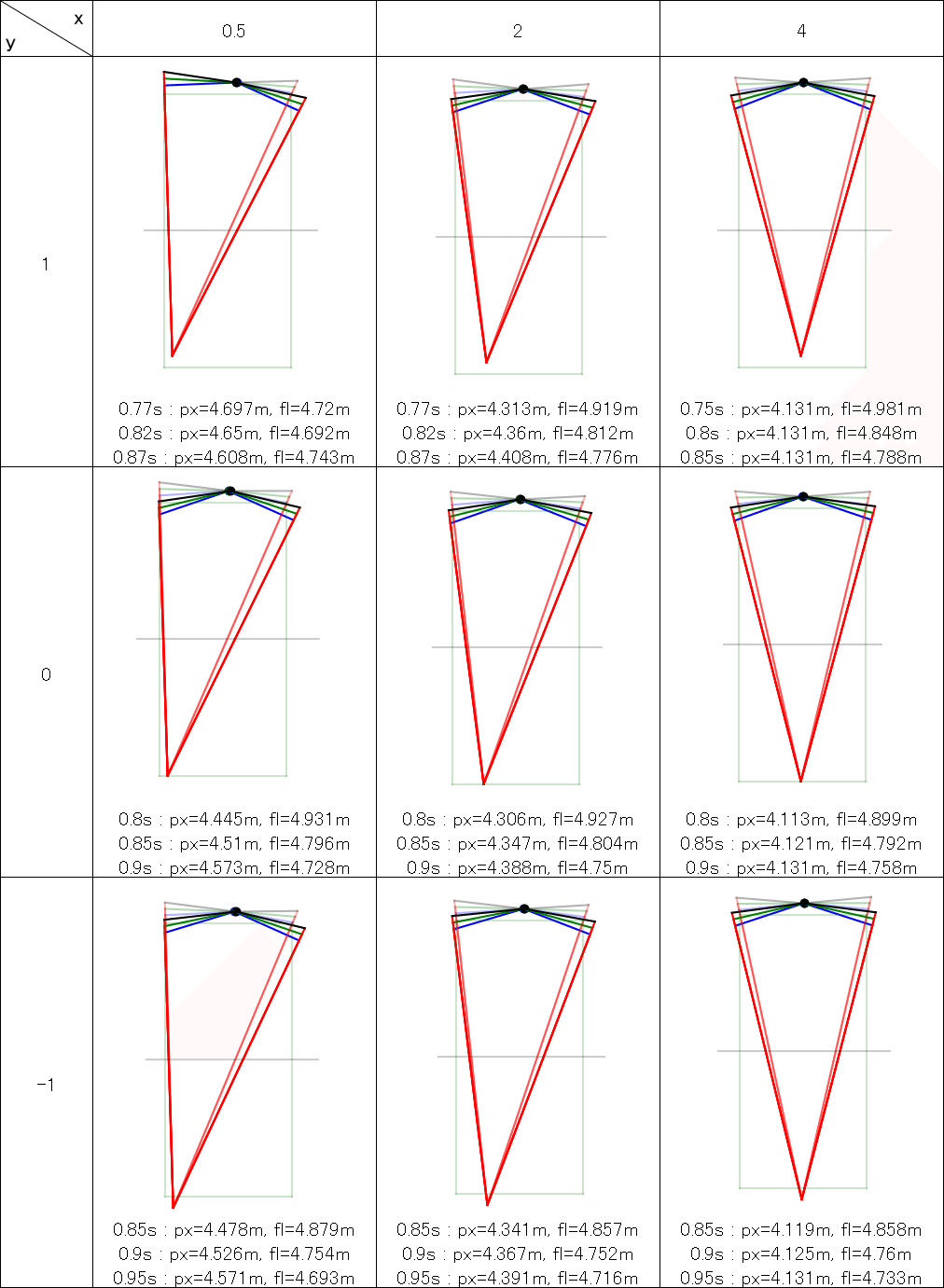
相手のヒッティングポジションは、横はサイドライン付近(x=0.5)、半面の中間(x=2)、センター付近(x=4)と、縦はベースライン内(y=1)、ベースライン上(y=0)、ベースライン後方(y=-1)を組み合わせた3×3の9パターン
下の数値は、{ショット到達時間 : 合理的待機位置のX座標(サイドラインからの距離), 合理的待機位置からの最長移動距離(一番外側のショットへの移動距離)}を表す
コート奥側の丸が合理的待機位置を表す
合理的待機位置から伸びている青、緑、黒線は、図の下にある合理的待機位置からの最長移動距離と一致する(上から順に、青、緑、黒線と対応する)
100km/h

110km/h

120km/h

130km/h

140km/h

150km/h
160km/h

170km/h

まとめ
今回は、相手のショットスピード・ポジション別に、合理的待機位置がどのように変化するかをみてみました。
最後までお読みいただきありがとうございました。
ご意見ご感想あれば、コメントにお願いします。