書記が数学やるだけ#787 ギブスサンプリング,メトロポリス-ヘイスティング法

マルコフ連鎖モンテカルロ法の例として,ギブスサンプリングとメトロポリス-ヘイスティング法を見ていく。
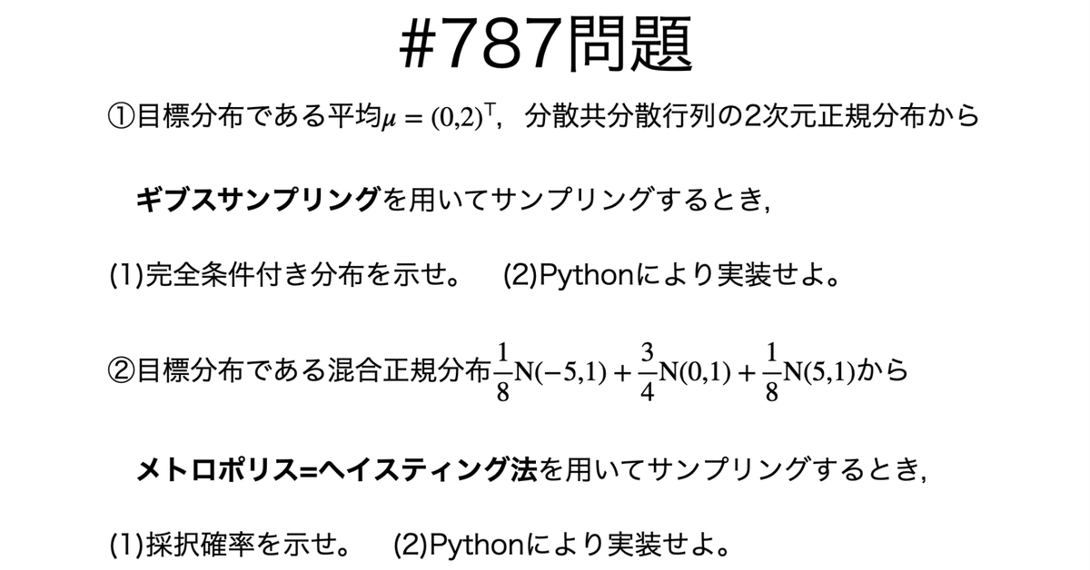
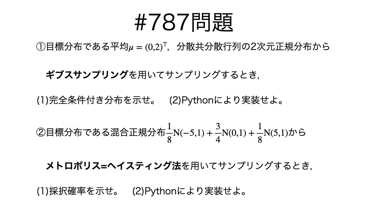
問題
説明
マルコフ連鎖について復習:
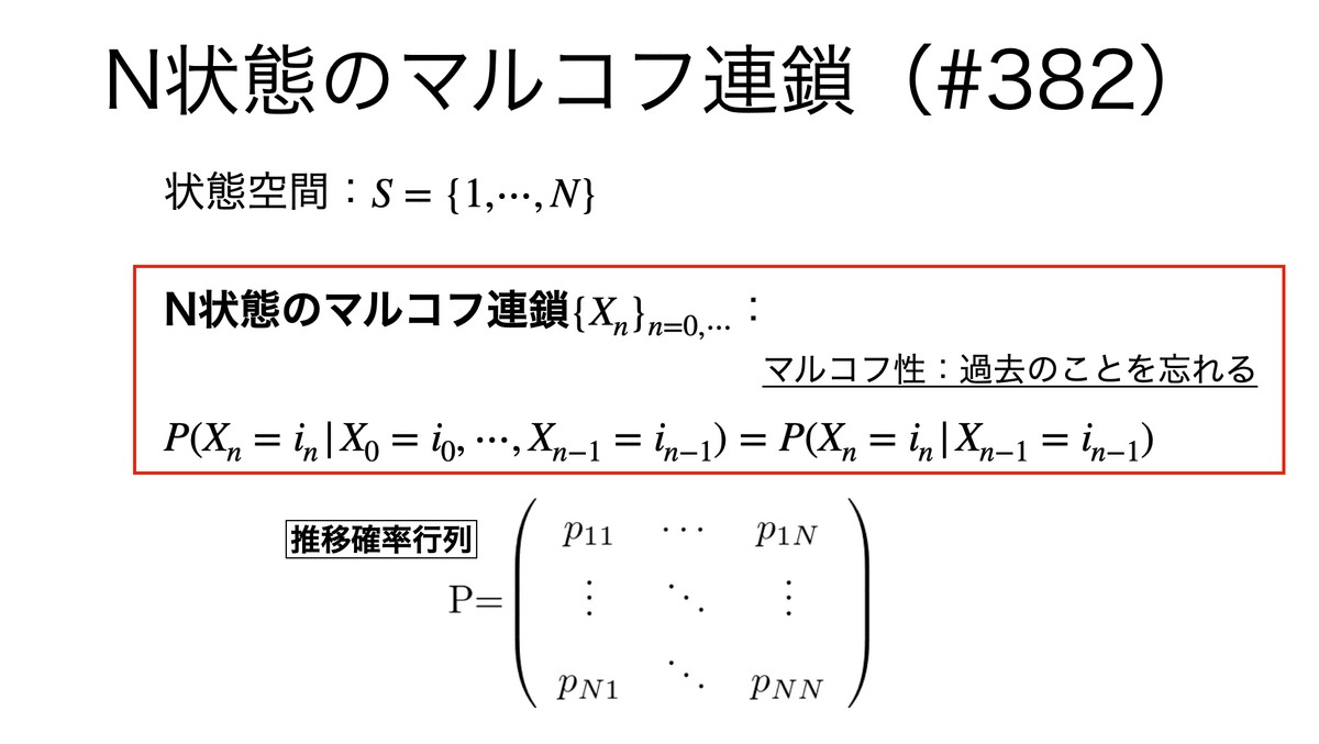
マルコフ連鎖モンテカルロ法(MCMC)とは,求める確率分布を均衡分布として持つマルコフ連鎖を作成することによって確率分布のサンプリングを行う種々のアルゴリズムの総称である。
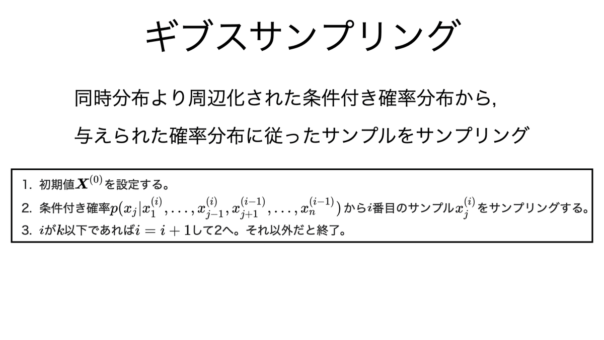
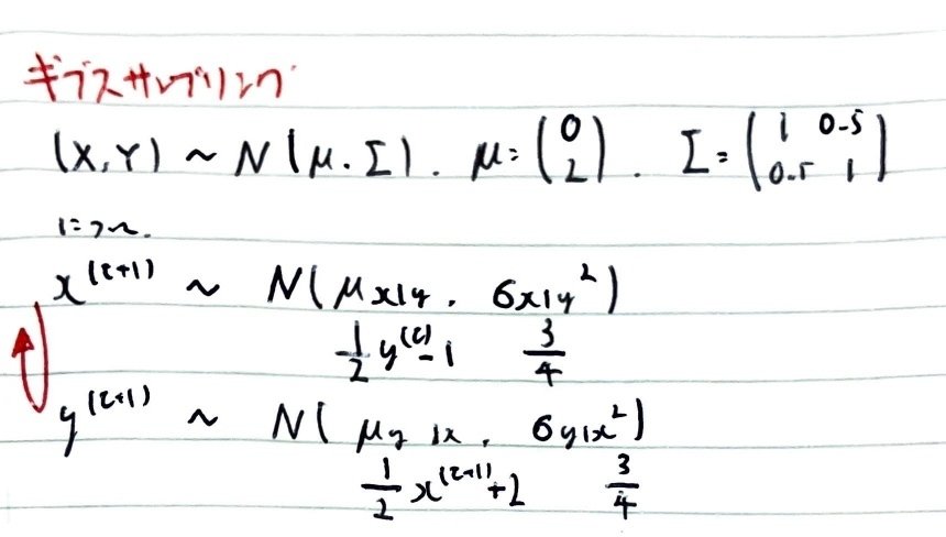
ギブスサンプリングでは,同時分布より周辺化された条件付き確率分布から与えられた確率分布に従ったサンプルをサンプリングする。
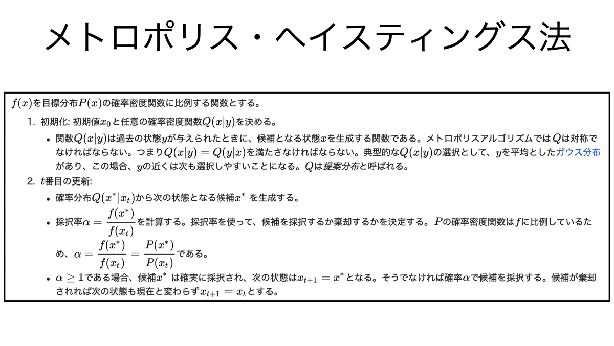
メトロポリス・ヘイスティングス法では,提案分布によりランダムウォークの粒子が次に移動する候補点を提案することで乱数列を生成する。
解答
ギブスサンプリングにおいて,周辺化された条件付き確率分布さえ求められれば計算ができる。
まず目標分布を作図しておく。
import numpy as np
from scipy import stats
import matplotlib.pyplot as plt

#目標分布
mu_x, mu_y = 0.0, 2.0
sigma_x, sigma_y = 1.0, 1.0
rho = 0.5

#平均
mus = np.array([mu_x, mu_y])
#分散共分散行列
sigmas = np.array([[sigma_x2, rhosigma_xsigma_y],
[rhosigma_xsigma_y, sigma_y2]])

x = np.arange(-4.0, 4.0, 0.1)
y = np.arange(-2.0, 6.0, 0.1)
X, Y = np.meshgrid(x, y)
pos = np.dstack((X, Y))
Z = stats.multivariate_normal.pdf(pos, mean=mus, cov=sigmas)

#等高線
fig, ax = plt.subplots(figsize=(12, 9))
cntr = ax.contour(X, Y, Z)
ax.clabel(cntr, fontsize=15)
plt.figure()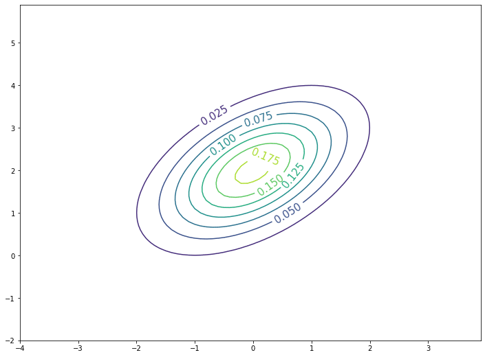
ギブスサンプリングは以下のように漸化式を組むことで実装できる。
#ギブスサンプリング
T = 10000
x_init=[0, 0]
samples = [x_init]
x, y = x_init[0], x_init[1]
for t in range(T):
    x = np.random.normal(1/2 * y -1, 3/4)
    samples.append([x, y])
    y = np.random.normal(1/2 * x +2, 3/4)
    samples.append([x, y])
ギブスサンプリングの結果を図示すると,確かに目標分布に沿ってサンプリングできていることがわかる。
fig, ax = plt.subplots(figsize=(12, 9))

#ギブスサンプリングの点
ax.scatter([row[0] for row in samples], [row[1] for row in samples], alpha=0.15, c='g')
#ギブスサンプリングの軌道(最初から100サイクルまで)
ax.plot([row[0] for row in samples][:100], [row[1] for row in samples][:100], c='r')
#初期位置
ax.plot(x_init[0], x_init[1], marker='.', ms=15, c='k')

cntr = ax.contour(X, Y, Z)
ax.clabel(cntr, fontsize=15)
plt.figure()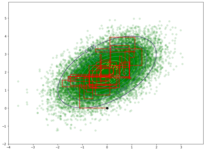
次にメトロポリス-ヘイスティング法について,実装では採択確率が重要になってくる。
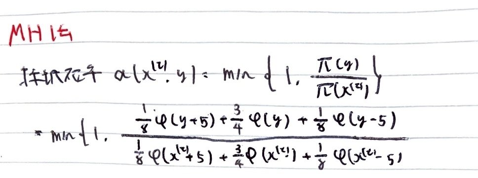
メトロポリス-ヘイスティング法の実装において,採択するか否かはif文で記述できる。
#メトロポリス-ヘイスティング法
T = 10000
x_data = np.zeros(T)
x_data[0] = 0

for t in range(1, T):
    y = x_data[t-1] + np.random.uniform(-10, 10)
    u = np.random.rand()
    #採択確率
    a = (1/8)*norm.pdf(y+5) + (3/4)*norm.pdf(y) + (1/8)*norm.pdf(y-5)
    b = (1/8)*norm.pdf(x_data[t]+5) + (3/4)*norm.pdf(x_data[t]) + (1/8)*norm.pdf(x_data[t]-5)
    alpha = min(1, a/b)
    #採択するか否か
    if u <= alpha:
        x_data[t] = y
    else:
        x_data[t] = x_data[t-1]

#サンプリングの軌道
plt.figure(figsize=(12, 8))
plt.plot(x_data)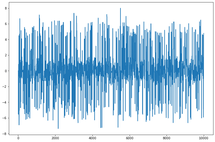
結果を照らし合わせてみると,確かにサンプリングできていることがわかる。
#サンプリングの結果
plt.hist(x_data, bins = 20, density = True)
#目標分布
x = np.arange(-10.,10.01,0.01)
f_x = 0.1stats.norm.pdf(x,-5,1) + 0.75stats.norm.pdf(x,0,1) + 0.1*stats.norm.pdf(x,5,1)
plt.plot(x,f_x,color="r")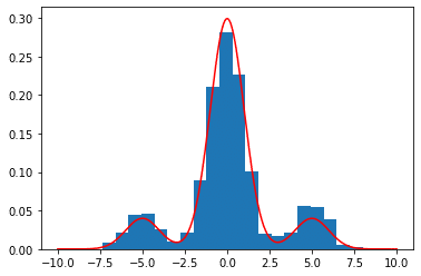
本記事のもくじはこちら: