
Re:ゲーム理論入門 プログラミング第1回 〜PythonでNash均衡をミル ~

みなさん、こんにちは、こんばんは。S.Kと申します。
今回はタイトルの通りPythonでNash均衡を見てみます。
「見る」ということなので求めてるわけではなく、単に手計算の結果を確認するために作成されたものです。(その点はご承知ください)
考える利得表(2人ゲーム、かつ2戦略×2戦略の利得表)
赤枠は純戦略におけるナッシュ均衡です。

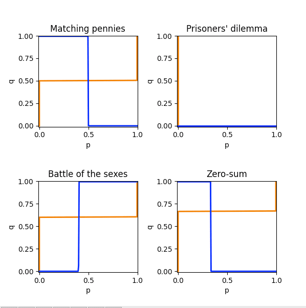
結果
交点がナッシュ均衡です。
おまけ
こちらの動画で作っていたものを流用しています。だいぶ前に作ったものです。
プログラム
細かいとこは端折りますが、相手の混合戦略に対して最適(利得が大きくなるところ)を求めて、図示してます。
デバッグしてないのでもしかしたらバグがあるかも・・・汗
import numpy as np
import matplotlib.pyplot as plt

payoff_matrix = []

# ペニー合わせ
payoff_matrix.append(np.array([[[1, -1], [-1, 1]], \
                         [[-1, 1], [1, -1]]]))

# 囚人のジレンマ
payoff_matrix.append(np.array([[[2, 2], [-1, 3]], \
                          [[3, -1], [1, 1]]]))

# 男女の争い
payoff_matrix.append(np.array([[[2, 3], [0, 0]], \
                        [[0, 0], [3, 2]]]))

# ゼロ和ゲーム
payoff_matrix.append(np.array([[[2, -2], [-2, 2]], \
                          [[0, 0], [2, -2]]]))

def function_0(q, x):
   if q.size == 0:
       print("test")
   else:
       pass

   P = np.empty([q.size,])
   retP = np.empty([q.size,])

   for idx in range(0, q.size, 1):
       for num in range(0, q.size, 1):
           temp_p = num / q.size
           P[num] = temp_p*q[idx]*x[0, 0, 0]\
           + temp_p*(1-q[idx])*x[0, 1, 0]\
           + (1-temp_p)*q[idx]*x[1, 0, 0]\
           + (1-temp_p)*(1-q[idx])*x[1, 1, 0]

       retP[idx] = np.argmax(P) / q.size

   return retP

def function_1(p, x):
   if p.size == 0:
       print("test")
   else:
       pass

   Q = np.empty([p.size,])
   retQ = np.empty([p.size,])

   for idx in range(0, p.size, 1):
       for num in range(0, p.size, 1):
           temp_q = num / p.size
           Q[num] = p[idx]*temp_q*x[0, 0, 1]\
           + p[idx]*(1-temp_q)*x[0, 1, 1]\
           + (1-p[idx])*temp_q*x[1, 0, 1]\
           + (1-p[idx])*(1-temp_q)*x[1, 1, 1]

       retQ[idx] = np.argmax(Q) / p.size

   return retQ

fig = plt.figure(figsize=(6, 6)) #グラフ描画領域
ax = []

#最適反応曲線がy軸と被ってm見えなくなってしまうので-0.01に設定
ax.append(fig.add_subplot(2, 2, 1, title='Matching pennies', xlim=(-0.01, 1), ylim=(-0.01, 1)))
ax.append(fig.add_subplot(2, 2, 2, title='Prisoners\' dilemma', xlim=(-0.01, 1), ylim=(-0.01, 1)))
ax.append(fig.add_subplot(2, 2, 3, title='Battle of the sexes', xlim=(-0.01, 1), ylim=(-0.01, 1)))
ax.append(fig.add_subplot(2, 2, 4, title='Zero-sum', xlim=(-0.01, 1), ylim=(-0.01, 1)))

mixed_range = [[np.arange(0, 1, 0.005)] * 2 for j in range(4)]

for j in range(4):
   # 確認用
   print(payoff_matrix[j])

   BR_P = function_0(mixed_range[j][1], payoff_matrix[j])
   BR_Q = function_1(mixed_range[j][0], payoff_matrix[j])
   ax[j].plot(BR_P, mixed_range[j][0], linestyle = "solid", linewidth = 2, color='#ee7800')
   ax[j].plot(mixed_range[j][1], BR_Q, linestyle = "solid", linewidth = 2, color='b')
   ax[j].set_xlabel("p")
   ax[j].set_ylabel("q")

plt.subplots_adjust(wspace=0.4, hspace=0.6)
with plt.style.context('classic'):
       plt.show()
参考文献
いつもの;
入門:
Python基本
活動費、テキスト購入費に充てたいと思います。宜しくお願い致します。