
【Python】円経路に拘束された質点の運動シミュレーション

前回導出した経路に拘束された質点運動をシミュレーションするための計算アルゴリズムを用いた実際の例として円経路を取り上げるよ。計算に必要な経路に関する各種ベクトル(経路ベクトル・接線ベクトル・曲率ベクトル)の導出から始めるよ。
円経路の経路ベクトル・接線ベクトル・曲率ベクトル
そもそも円とは2次元平面上において、ある点からの距離が等距離となる点の集合で定義される図形だね。中心座標$${(x_0, y_0)}$$、半径$${r}$$の円を表す式は以下のとおりだね。
$$
(x-x_0)^2+(y-y_0)^2=r^2
$$
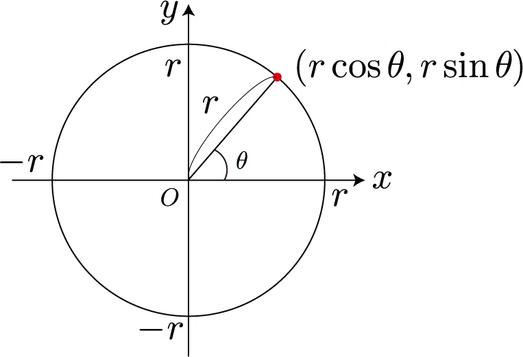
原点を中心とした円周上の任意の点は、媒介変数\thetaを用いて次のとおり与えられるね。
$$
\left\{ \begin{matrix}x(\theta )=r\cos \theta\\ y(\theta )=r\sin \theta\end{matrix} \right.
$$
これは2次元の極座標形式と同じだね。この媒介変数表示において、$${\theta=0}$$を始点、$${\theta=2\pi}$$を終点とした経路を経路ベクトル$${\boldsymbol{r}_{\rm path} (\theta)}$$と定義するね。前項で示した方法を適用して接線ベクトルと曲率ベクトルの導出していくよ。まず、これらのベクトル量の計算に必要な$${\theta}$$の$${l}$$の微分は
$$
\frac{d l}{d\theta } =r \ \to \ \frac{d \theta}{d l} =\frac{1}{r} \ , \ \frac{d^2 \theta}{d l^2} =0
$$
と得られるよ。円経路の接線ベクトルと曲率ベクトルはそれぞれ次のようになるね。
円経路の接線ベクトル
$$
\boldsymbol{t}_{\rm path} (\theta)= \frac{1}{r} (-r\sin \theta ,r\cos\theta) = (-\sin \theta ,\cos\theta)
$$
円経路の曲率ベクトル
$$
\boldsymbol{\chi} (\theta) = \frac{1}{r^2}\,(-r\cos\theta, -r\sin\theta )= -\frac{1}{r} \,(\cos\theta, \sin\theta )
$$
ちなみに曲率ベクトルを媒介変数表示の経路ベクトル\$${\boldsymbol{r}_{\rm path} (\theta)}$$を用いると
$$
\boldsymbol{\chi} (\theta) = - \frac{1}{r^2} \, \boldsymbol{r}_{\rm path} (\theta)
$$
となるね。さっそく計算結果を示すよ。最後の方は目の錯覚が起きるね。
Pythonプログラムソース
上記のシミュレーションを行うプログラムソースを公開するよ。もしよかったら試してみてください。これからも応援してください。よろしくお願いしまーす!
#################################################################
TITLE = "経路に拘束された運動(円経路)"
#################################################################
import os
import numpy as np
import scipy.integrate as integrate
import matplotlib.pyplot as plt
import matplotlib.animation as animation
import colorsys
###############################
# 実験室グローバル変数
###############################
TIME_START = 0.0        #計算開始時刻
TIME_END   = 10.0       #計算終了時刻
DT = 0.01               #時間間隔
PLOT_FLAG = False        #グラフ描画
ANIMATION_FLAG = True  #アニメーション作成
ANIMATION_INTERVAL = 5 #アニメーション作成時の描画インターバル
OUTPUT_FLAG = False
OUTPUT_PASS = "./data_20241101/"
if( OUTPUT_FLAG and os.path.isdir(OUTPUT_PASS) == False) : os.mkdir(OUTPUT_PASS)
###############################
# 計算グローバル変数
###############################
#時刻
times = np.arange(TIME_START, TIME_END, DT)
#重力加速度
vec_g = np.array([0, 0, -10])
#質量
m = 1.0

#初速度の大きさ
v0s = np.arange(0.02, 0.05+0.0001, 0.0001)
###############################
# 関数定義
###############################
#相対誤差
rtol = 1e-9
#絶対誤差
atol = 1e-9


# 経路の設定
class Path:
	#コンストラクタ
	def __init__(self):
		#円の半径
		self.R = 1
		#円の中心位置ベクトル
		self.center = np.array([0.0, 0.0, self.R])

	#経路の位置ベクトルを指定する媒介変数関数
	def position( self, theta ):
		x = self.R * np.cos(theta)
		y = 0
		z = self.R * np.sin(theta) + self.center[2]
		return np.array([x, y, z])

	#接線ベクトルを指定する媒介変数関数
	def tangent( self, theta ):
		x = -np.sin(theta)
		y = 0
		z = np.cos(theta)
		return np.array([x, y, z])
	#曲率ベクトルを指定する媒介変数関数
	def curvature( self, theta ):
		x = -np.cos(theta) / self.R
		y = 0
		z = -np.sin(theta) / self.R
		return np.array([x, y, z])
	#媒介変数の取得
	def getTheta( self, r ):
		#相対位置ベクトル
		bar_r = r - self.center
		bar_r_length = np.sqrt(np.sum( bar_r**2 ))
		sinTheta = bar_r[2] / bar_r_length
		if( sinTheta > 0 ):
			theta = np.arccos( bar_r[0] / bar_r_length )
		else:
			theta = 2.0 * np.pi - np.arccos( bar_r[0] / bar_r_length )

		return theta


#経路拘束力の微分方程式
def equations(t, X, path, vec_g):
	vec_r =  np.array([ X[0], X[1], X[2] ])
	vec_v =  np.array([ X[3], X[4], X[5] ])

	#媒介変数の取得
	theta = path.getTheta ( vec_r )

	#媒介変数に対する位置ベクトル、接線ベクトル、曲率ベクトルの計算
	position = path.position( theta )
	tangent = path.tangent( theta )
	curvature = path.curvature( theta )

	#経路中心の位置ベクトル・速度ベクトル・加速度ベクトル
	vec_r_box = np.copy( path.center )
	vec_v_box = np.array([0.0, 0.0, 0.0])
	vec_a_box = np.array([0.0, 0.0, 0.0])

	#相対速度
	bar_v = vec_v - vec_v_box

	#微係数dl/dtとd^2l/dt^2を計算
	dl_dt = np.dot( bar_v, tangent )
	d2l_dt2 = np.dot( vec_g, tangent ) - np.dot( vec_a_box, tangent)

	#加速度を計算
	vec_a = vec_a_box + d2l_dt2 * tangent + dl_dt * dl_dt * curvature

	return [vec_v[0], vec_v[1], vec_v[2], vec_a[0], vec_a[1], vec_a[2]]

# 初速度依存性を可視化
def calculation(vec_r0, vec_v0, path, vec_g):

	solution = integrate.solve_ivp(
		equations,                     #常微分方程式
		method = 'RK45',                #計算方法
		args = (path, vec_g),              #引数
		t_span=( times[0], times[-1]),  #積分区間
		rtol = rtol,                   #相対誤差
		atol = atol,                   #絶対誤差
		y0 = np.concatenate([vec_r0, vec_v0]), #初期値
		t_eval = times                  #結果を取得する時刻
	)
	#計算結果
	return solution.y[ 0 ], solution.y[ 1 ], solution.y[ 2 ], solution.y[ 3 ], solution.y[ 4 ], solution.y[ 5 ]

##########################################################
if __name__ == "__main__":

	#経路の生成
	path = Path()
	#描画用リスト
	xls = []
	yls = []
	zls = []
	vxls = []
	vyls = []
	vzls = []
	#theta による違い
	for i in range(len(v0s)):
		print( i )

		#初期位置と速度
		vec_r0 = np.array([ 0, 0, 2 ])
		vec_v0 = np.array([ v0s[i], 0, 0])

		x, y, z, vx, vy, vz = calculation( vec_r0, vec_v0, path, vec_g )
		xls.append( x )
		yls.append( y )
		zls.append( z )
		vxls.append( vx )
		vyls.append( vy )
		vzls.append( vz )

		vec_r = np.array([ x[-1], y[-1], z[-1] ])
		vec_v = np.array([ vx[-1],vy[-1],vz[-1] ])

		E_start = 1.0/2.0 * m * np.sum( vec_v0**2 ) - m * np.dot( vec_g, vec_r0 )
		E_end =   1.0/2.0 * m * np.sum( vec_v**2 )  - m * np.dot( vec_g, vec_r )
		DeltaE = np.abs(E_end - E_start)
		print( E_start, E_end, " |ΔE/E(0)| =", DeltaE / E_start )

	if( OUTPUT_FLAG ):
		for i in range(len(times)):
			f_path = OUTPUT_PASS + str( i ) + '.txt'
			f = open(f_path, 'w')

			for j in range( len(xls) ):
				f.write( str(round( xls[ j ][ i ], 4)) + "\t" +  str(round( yls[ j ][ i ], 4)) + "\t" + str(round( zls[ j ][ i ], 4)) + "\t" +  str(round( vxls[ j ][ i ], 4)) + "\t" + str(round( vyls[ j ][ i ], 4)) + "\t" +  str(round( vzls[ j ][ i ], 4)) + "\n")

			f.close()

	if( PLOT_FLAG ):
		#################################################################
		# グラフの設定
		#################################################################
		fig = plt.figure( figsize=(12, 8) ) #画像サイズ
		plt.subplots_adjust(left = 0.085, right = 0.97, bottom = 0.10, top = 0.95) #グラフサイズ
		plt.rcParams['font.family'] = 'Times New Roman' #フォント
		plt.rcParams['font.size'] = 16 #フォントサイズ
		plt.rcParams["mathtext.fontset"] = 'cm' #数式用フォント
		#カラーリストの取得
		colors = plt.rcParams['axes.prop_cycle'].by_key()['color']
		#グラフタイトルと軸ラベルの設定
		plt.title( TITLE, fontname="Yu Gothic", fontsize=20, fontweight=500 )
		plt.xlabel( r"$t \,[{\rm s}]$", fontname="Yu Gothic", fontsize=20, fontweight=500 )
		plt.ylabel( r"$z \,[{\rm m}]$" , fontname="Yu Gothic", fontsize=20, fontweight=500 )
		#罫線の描画
		plt.grid( which = "major", axis = "x", alpha = 0.7, linewidth = 1 )
		plt.grid( which = "major", axis = "y", alpha = 0.7, linewidth = 1 )

		#描画範囲を設定
		plt.xlim([0, TIME_END])
		plt.ylim([0, 2])

		#グラフの描画
		for i in range(len(v0s)):
			c = colorsys.hls_to_rgb( i/len(v0s) , 0.5 , 1)
			plt.plot(times, zls[i], linestyle='solid', linewidth = 4)#, color = c)

		#グラフの表示
		plt.show()

	if( ANIMATION_FLAG ):

		#円座標点配列の生成
		thetas = np.linspace(0, 2*np.pi, 200)
		cirsx = np.cos( thetas )
		cirsy = np.sin( thetas ) + 1.0

		#################################################################
		# アニメーションの設定
		#################################################################
		fig = plt.figure(figsize=(8, 8)) #画像サイズ
		plt.subplots_adjust(left = 0.07, right = 0.98, bottom = 0.07, top = 0.95) #グラフサイズ
		plt.rcParams['font.family'] = 'Times New Roman' #フォント
		plt.rcParams['font.size'] = 16 #フォントサイズ
		plt.rcParams["mathtext.fontset"] = 'cm' #数式用フォント
		#カラーリストの取得
		colors = plt.rcParams['axes.prop_cycle'].by_key()['color']

		#アニメーション作成用
		imgs = []

		#アニメーション分割数
		AN = len( times )

		#軌跡リスト
		r_trajectorys = [ 0.0 ] * len( v0s )

		#アニメーションの各グラフを生成
		for an in range( AN ):
			t = DT * an

			if( an % ANIMATION_INTERVAL != 0): continue

			#軌跡の描画
			img = plt.plot(cirsx, cirsy, color = "black", linestyle='dotted', linewidth = 1 )

			for i in range( len( v0s ) ):
				c = colorsys.hls_to_rgb( i/len(v0s) , 0.5 , 1)
				if( i == 0 ):
					img += plt.plot([xls[i][an]], [zls[i][an]], color = c, marker = 'o', markersize = 20)
				else:
					img += plt.plot([xls[i][an]], [zls[i][an]], color = c, marker = 'o', markersize = 20)


			#時刻をグラフに追加
			time = plt.text(13.5, 0.35, "t = " +  str("{:.2f}".format(t)), fontsize=18)
			img.append( time )

			imgs.append( img )

		#グラフタイトルと軸ラベルの設定
		plt.title( TITLE, fontname="Yu Gothic", fontsize=20, fontweight=500 )
		#plt.xlabel( r"$x \,[{\rm m}]$", fontname="Yu Gothic", fontsize=20, fontweight=500 )
		#plt.ylabel( r"$z \,[{\rm m}]$" , fontname="Yu Gothic", fontsize=20, fontweight=500 )
		#罫線の描画
		plt.grid( which = "major", axis = "x", alpha = 0.7, linewidth = 1 )
		plt.grid( which = "major", axis = "y", alpha = 0.7, linewidth = 1 )

		#描画範囲を設定
		plt.xlim([-1.2, 1.2])
		plt.ylim([-0.2, 2.2])
		#アニメーションの生成
		ani = animation.ArtistAnimation(fig, imgs, interval=50)
		#アニメーションの保存
		ani.save("output.html", writer=animation.HTMLWriter())
		#ani.save("output.gif", writer="imagemagick")
		#ani.save("output.mp4", writer="ffmpeg", dpi=360)
		#グラフの表示
		#plt.show()