
Pythonで採用データの可視化 積み立てグラフ、折れ線グラフを描画するスクリプト

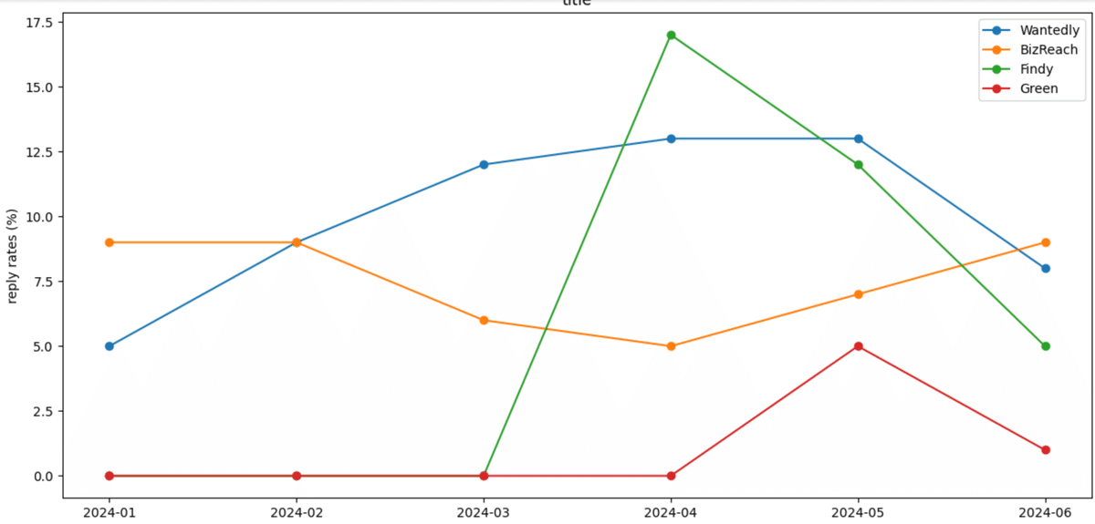
折れ線グラフ描画のスクリプト
Google Colabでコピペで試すことが出来ます。
import matplotlib.pyplot as plt

def plot_media_reply_rates(media_reply_rates_by_month, ax2):
    # 媒体と月の組み合わせを取得
    media_list = list(media_reply_rates_by_month.keys())
    month_list = sorted(set(month for media_rates in media_reply_rates_by_month.values() for month, _ in media_rates))

    print(f'\nmedia_list:\n{media_list}\n')
    print(f'\nmonth_list:\n{month_list}\n')

    # 折れ線グラフの描画
    for media in media_list:
        rates = {month: rate for month, rate in media_reply_rates_by_month[media]}
        plot_data = [rates.get(month, 0) for month in month_list]

        print(f'\nmedia: {media}')
        print(f'rates:\n{rates}')
        print(f'plot_data:\n{plot_data}\n')

        ax2.plot(month_list, plot_data, marker='o', label=media)

    # ax2.set_xlabel('月')
    ax2.set_ylabel('reply rates (%)')
    ax2.set_title('title')
    ax2.legend()
    plt.xticks(rotation=0)
    plt.tight_layout()

# 使用例
fig, ax = plt.subplots(figsize=(12, 6))
media_reply_rates_by_month = {'Wantedly': [('2024-01', 0), ('2024-02', 9), ('2024-03', 12), ('2024-04', 13), ('2024-05', 33), ('2024-06', 8)], 'BizReach': [('2024-01', 9), ('2024-02', 9), ('2024-03', 6), ('2024-04', 5), ('2024-05', 7), ('2024-06', 9)], 'Findy': [('2024-04', 31), ('2024-05', 12), ('2024-06', 0)], 'Green': [('2024-05', 5), ('2024-06', 1)]}

print(f'\nmedia_reply_rates_by_month:\n{media_reply_rates_by_month}\n')

plot_media_reply_rates(media_reply_rates_by_month, ax)
plt.show()
折れ線の装飾について
ax2.plot(month_list, plot_data, marker='o', label=media)受け取れる引数について
markeredgecolor='white' # 点を強調するための色
color=’#cccccc’ # 線の色
label=f'{media}の返信率', # グラフの凡例
linewidth=1.25 # 線の太さ
linestyle='--' # 破線、ハッチング、ストライプなどを指定できる
採用媒体別の色の割り当て
color_map = {
    'ビズリーチ': '#0b2787',
    'Wantedly': '#21bddb',
    'Green': '#60b630',
    'Findy': '#109f95',
    'YOUTRUST': '#279fa8'
}
横並び積み上げ棒グラフ
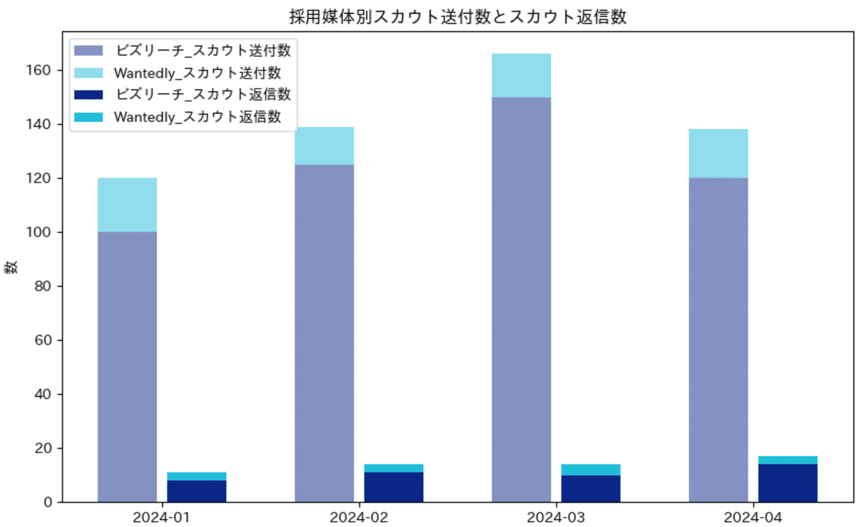
横並び積み上げ棒グラフ?とでも言うのでしょうか?
1月という一つのindexに2つの棒グラフを描画します。
!pip install -q japanize_matplotlib上記の記述で、日本語表記が出来るようになります!!
import pandas as pd
import japanize_matplotlib
import matplotlib.pyplot as plt
import numpy as np

# データフレームの作成
data = {
    'ビズリーチ_スカウト送付数': [100, 125, 150, 120],
    'ビズリーチ_スカウト返信数': [8, 11, 10, 14],
    'Wantedly_スカウト送付数': [20, 14, 16, 18],
    'Wantedly_スカウト返信数': [3, 3, 4, 3]
}

# インデックスを設定してデータフレームを作成
df = pd.DataFrame(data, index=['2024-01', '2024-02', '2024-03', '2024-04'])

# プロットの設定
fig, ax = plt.subplots(figsize=(10, 6), sharey=True)

# バーの幅と間隔を設定
bar_width = 0.3
space_between_bars = 0.05

# インデックスの位置を設定
indices = np.arange(len(df.index))

# スカウト送付数の棒グラフをプロット
ax.bar(indices - bar_width/2 - space_between_bars/2, df['ビズリーチ_スカウト送付数'], bar_width, label='ビズリーチ_スカウト送付数', color='#0b2787', alpha=0.5)
ax.bar(indices - bar_width/2 - space_between_bars/2, df['Wantedly_スカウト送付数'], bar_width, bottom=df['ビズリーチ_スカウト送付数'], label='Wantedly_スカウト送付数', color='#21bddb', alpha=0.5)

# スカウト返信数の棒グラフをプロット
ax.bar(indices + bar_width/2 + space_between_bars/2, df['ビズリーチ_スカウト返信数'], bar_width, label='ビズリーチ_スカウト返信数', color='#0b2787')
ax.bar(indices + bar_width/2 + space_between_bars/2, df['Wantedly_スカウト返信数'], bar_width, bottom=df['ビズリーチ_スカウト返信数'], label='Wantedly_スカウト返信数', color='#21bddb')

# グラフのタイトルとラベルを設定
ax.set_title('採用媒体別スカウト送付数とスカウト返信数')
ax.set_xlabel('')
plt.xticks(indices, df.index)
ax.set_ylabel('数')

# 凡例を設定
ax.legend(loc='upper left')

# プロットの表示
plt.show()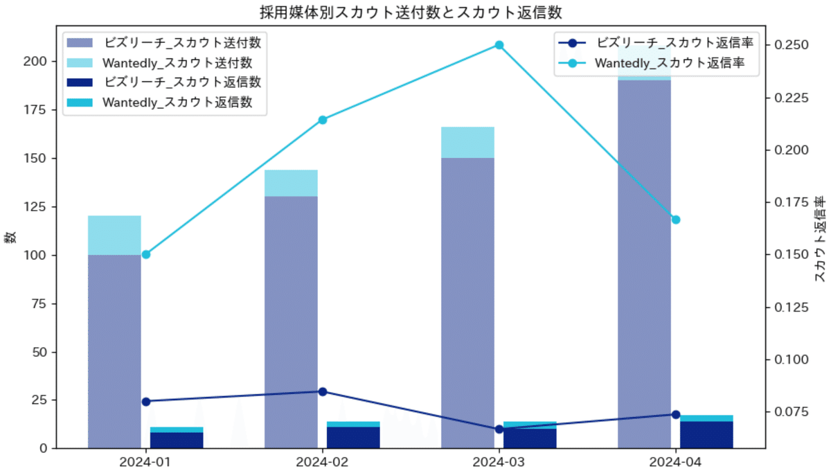
Chat GPTに作ってもらったコードですが、棒グラフと折れ線グラフを作るコードそれぞれ関数として分けた方が可読性は上がりそうですね。
import pandas as pd
import japanize_matplotlib
import matplotlib.pyplot as plt
import numpy as np

# データフレームの作成
data = {
    'ビズリーチ_スカウト送付数': [100, 130, 150, 190],
    'ビズリーチ_スカウト返信数': [8, 11, 10, 14],
    'Wantedly_スカウト送付数': [20, 14, 16, 18],
    'Wantedly_スカウト返信数': [3, 3, 4, 3]
}

# インデックスを設定してデータフレームを作成
df = pd.DataFrame(data, index=['2024-01', '2024-02', '2024-03', '2024-04'])

# スカウト返信率を計算
df['ビズリーチ_スカウト返信率'] = df['ビズリーチ_スカウト返信数'] / df['ビズリーチ_スカウト送付数']
df['Wantedly_スカウト返信率'] = df['Wantedly_スカウト返信数'] / df['Wantedly_スカウト送付数']

# プロットの設定
fig, ax = plt.subplots(figsize=(10, 6), sharey=True)
ax2 = ax.twinx()  # ax2を追加

# バーの幅と間隔を設定
bar_width = 0.3
space_between_bars = 0.05

# インデックスの位置を設定
indices = np.arange(len(df.index))

# スカウト送付数の棒グラフをプロット
ax.bar(indices - bar_width/2 - space_between_bars/2, df['ビズリーチ_スカウト送付数'], bar_width, label='ビズリーチ_スカウト送付数', color='#0b2787', alpha=0.5)
ax.bar(indices - bar_width/2 - space_between_bars/2, df['Wantedly_スカウト送付数'], bar_width, bottom=df['ビズリーチ_スカウト送付数'], label='Wantedly_スカウト送付数', color='#21bddb', alpha=0.5)

# スカウト返信数の棒グラフをプロット
ax.bar(indices + bar_width/2 + space_between_bars/2, df['ビズリーチ_スカウト返信数'], bar_width, label='ビズリーチ_スカウト返信数', color='#0b2787')
ax.bar(indices + bar_width/2 + space_between_bars/2, df['Wantedly_スカウト返信数'], bar_width, bottom=df['ビズリーチ_スカウト返信数'], label='Wantedly_スカウト返信数', color='#21bddb')

# スカウト返信率のプロット
ax2.plot(indices, df['ビズリーチ_スカウト返信率'], color='#0b2787', marker='o', label='ビズリーチ_スカウト返信率')
ax2.plot(indices, df['Wantedly_スカウト返信率'], color='#21bddb', marker='o', label='Wantedly_スカウト返信率')

# グラフのタイトルとラベルを設定
ax.set_title('採用媒体別スカウト送付数とスカウト返信数')
ax.set_xlabel('')
plt.xticks(indices, df.index)
ax.set_ylabel('数')
ax2.set_ylabel('スカウト返信率')  # ax2のy軸ラベルを設定

# 凡例を設定
ax.legend(loc='upper left')
ax2.legend(loc='upper right')  # ax2の凡例を設定

# プロットの表示
plt.show()