MATLAB で図形の境界データを検出する

まえがき
みなさん、毎年恒例、motorcontrolman さん主催の MATLAB/Simulink Advent Calendar 2024 楽しみましたか?
その中で WandererEng さんが、イラストの外形座標を取得するのに、MATLAB で画像を表示し、データヒント機能を使って手動でポイントをクリックしていく方法を紹介されていました。
データヒントは MATLAB の標準機能であり、最も手軽かつ汎用的に使える方法かと思います。
データヒント機能についてはこちらの記事でも紹介しています。
表示のカスタマイズや、スクリプトから操作することもできます。
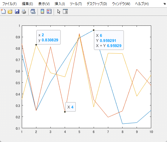
Image Toolbox で自動化
たまにやるくらいならデータヒントを使うのが最適かと思いますが、いくつも手動でやるのは大変です。
他人様のネタをネタにして、自動化を検討してみましょう。
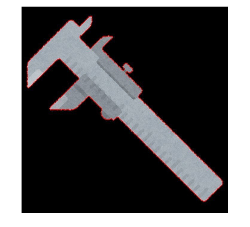
Image Toolbox には bwboundaries という境界をトレースする関数があります。
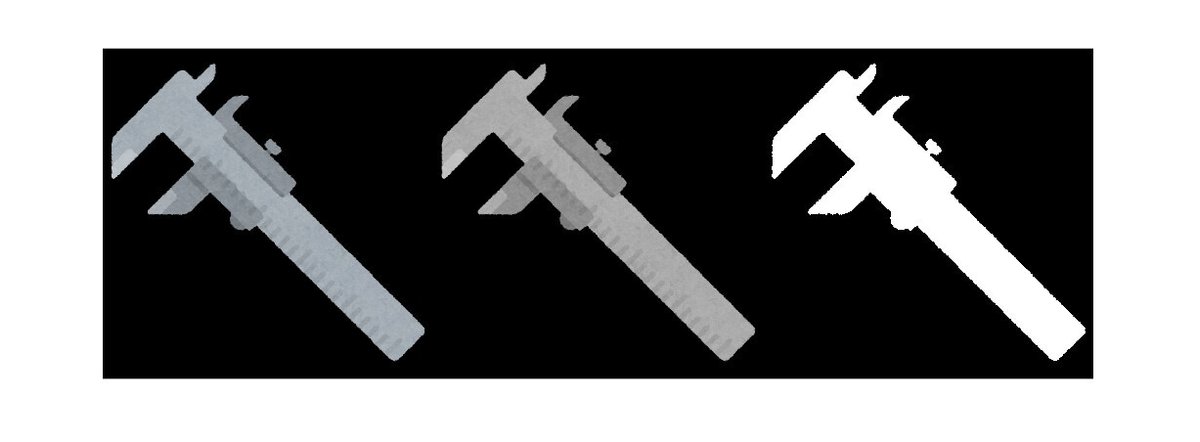
対象は2値画像のみなので、変換してから入力します。
img = imread('https://blogger.googleusercontent.com/img/b/R29vZ2xl/AVvXsEhDQ6v6yNnB6eS6LKAi7YcSFUgIWrxQorBjtPboeDq-dxjCiEc6yH3gQqbchhfJeacupSAV6Y7NwRCODenXDu-p8TiXIofSuALJbHCk2myFJDeOoHkwnfL2nk36Yj3YWTLLVzllESf8sHEy/s800/dougu_nogisu.png');
grayImg = rgb2gray(img);
bwImg = imbinarize(grayImg);
[B, L] = bwboundaries(bwImg, 'noholes', CoordinateOrder='xy');
boundary = B{1};
plot(boundary(:,1), -boundary(:,2));
axis equal
str = sprintf('%d points', length(boundary));
legend(str)
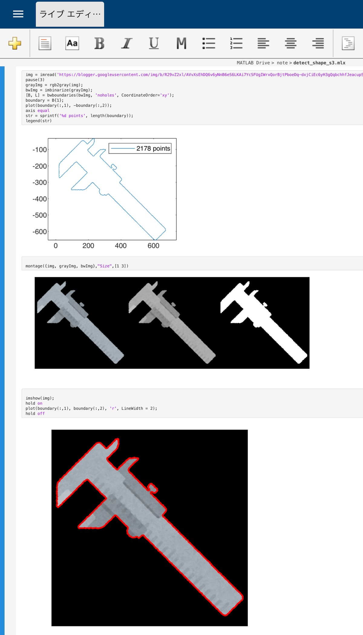
montage({img, grayImg, bwImg},"Size",[1 3])
imshow(img);
hold on
plot(boundary(:,1), boundary(:,2), 'r', LineWidth = 2);
hold off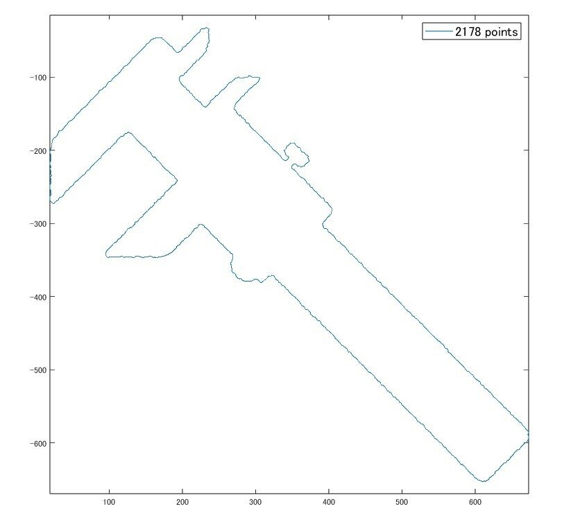
境界検出自体は1行でできます。
戻り値 B には検出された各領域の座標データが cell 形式で、L には背景を "0" とした、各領域毎に順番に振られたラベル番号が入っています。
イメージ系のY座標は下方向がプラスなので注意しましょう。
Image Toolbox は Online / Mobile 版無料アカウントでも使用することができます。
自分の iPhone、なぜか現在グラフィック関連がうまく動きません。(゚~゚)
ポイント数削減
別にこのままでも良いのですが、検出されたポイント数が2千個以上と多めです。
少し削減してみましょう。
傾きを計算して、基準点での傾きとの差が大きくなったときだけ境界点データを追加するようにしてみます。
boundary2 = boundary(1,:);
threshold = 1;

i1 = 1; % referrence point
for i = 2:length(boundary)-1
    diff1 = boundary(i1+1,:) - boundary(i1,:);
    diff2 = boundary(i+1,:) - boundary(i,:);

    diffMagnitude = norm(diff2 - diff1);

    if diffMagnitude > threshold
        i1 = i;  % update referrence point
        boundary2 = [boundary2; boundary(i,:)];
    end
end

plot(boundary2(:,1), -boundary2(:,2), '-o');
axis equal
str = sprintf('%d points', length(boundary2));
l = legend(str);
l.FontSize = 14;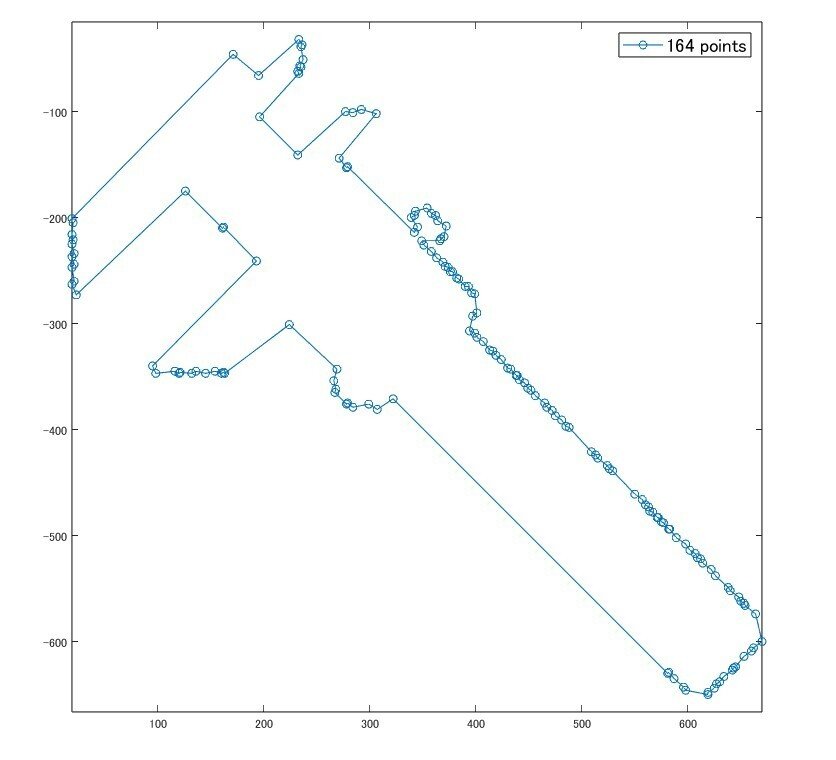
ほぼ形は保ったまま、2178 → 164 点に削減できました。
でもまだ、右下の直線に見える部分が結構詰まってますね。
拡大してみましょう。
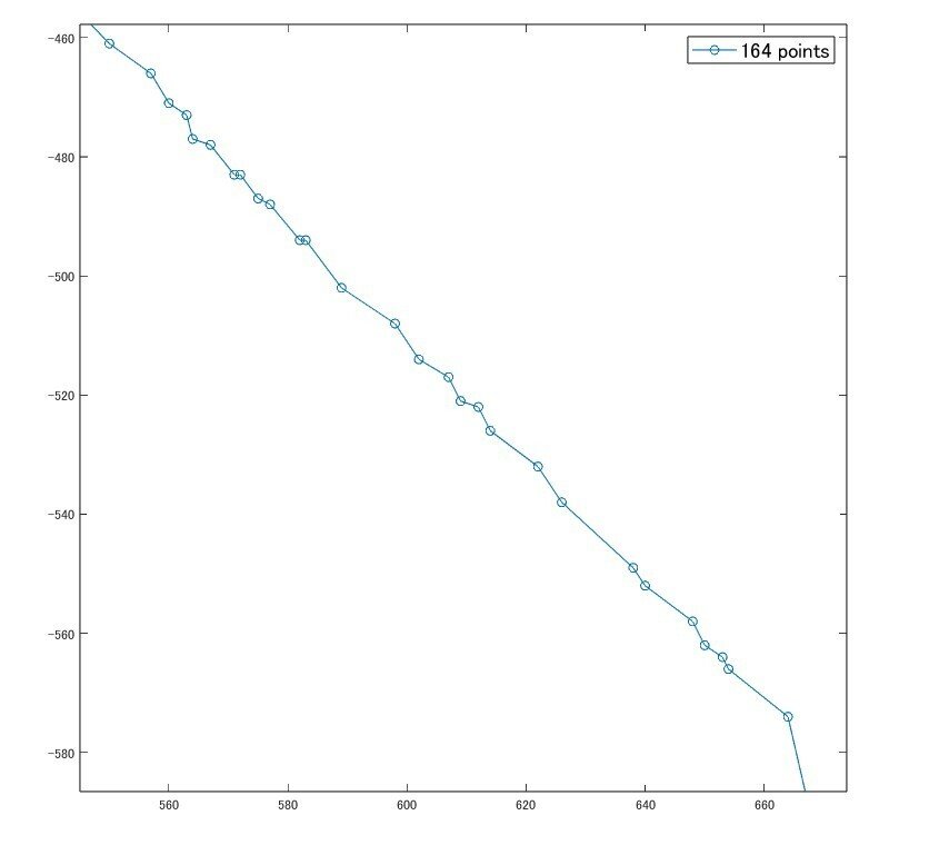
う~ん、割とガタガタしてますね。
前処理
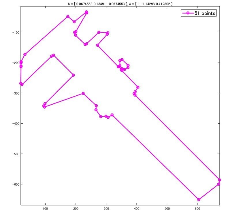
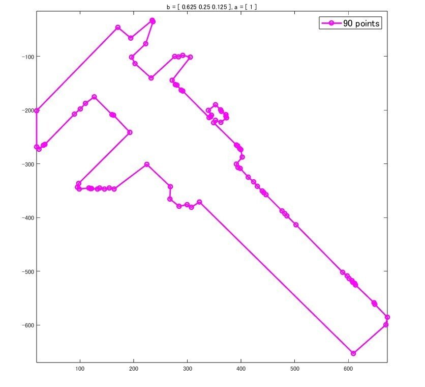
前処理として、LPF を掛けてみましょう。
何種類か試してみます。
フィルターを掛ける場合の注意点としては、端点処理があります。
そのまま掛けると、端点のデータがフィルターの影響を受けて変化してしまいます。
多くの場合0データを挿入したりもしますが、今回の場合は始点終点のデータを変えたくないので、padarray 関数を使ってフィルターの遅延分オーバーラップする形で元データを増やしてからフィルター処理をしています。
threshold = 1;

[b, a] = butter(2, .4);  n = length(b) * 2;
detShape(boundary, b, a, n, threshold)

[b, a] = butter(2, .2);  n = length(b) * 2;
detShape(boundary, b, a, n, threshold)

b = [.625 .25 .125];  a = 1; n = length(b);
detShape(boundary, b, a, n, threshold);

b = [.25 .5 .25];  a = 1;  n = length(b);
detShape(boundary, b, a, n, threshold);

n = 4; b = ones(1,n) / n;  a = 1;
detShape(boundary, b, a, n, threshold);


function points = detShape(boundary, b, a, n, threshold)
boundary_F0 = padarray(boundary,[n 0],'circular','both');
boundary_F = filter(b,a, boundary_F0);
boundary_F = boundary_F(n+1:end-n, :);

boundary2 = boundary_F(1,:);
i1 = 1; % referrence point
for i = 2:length(boundary_F)-1
    diff1 = boundary_F(i1+1,:) - boundary_F(i1,:);
    diff2 = boundary_F(i+1,:) - boundary_F(i,:);

    diffMagnitude = norm(diff2 - diff1);

    if diffMagnitude > threshold
        i1 = i;  % update referrence point
        boundary2 = [boundary2; boundary_F(i,:)];
    end
end
plot([boundary2(:,1); boundary2(1,1)], -[boundary2(:,2); boundary2(1,2)], 'm-o', LineWidth=2)
axis equal
str = sprintf('%d points', length(boundary2));
l = legend(str);
l.FontSize = 14;
end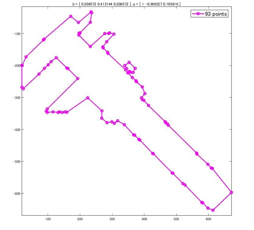
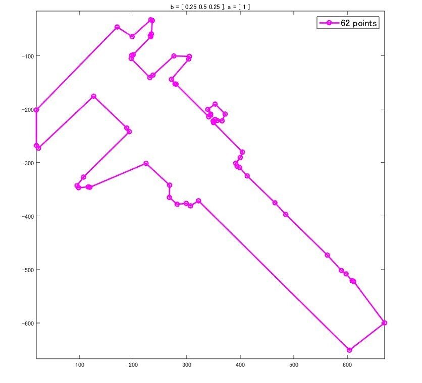
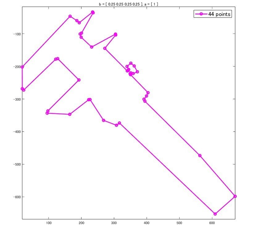
この辺りは元データの性質と目的に合わせて調整する必要があります。
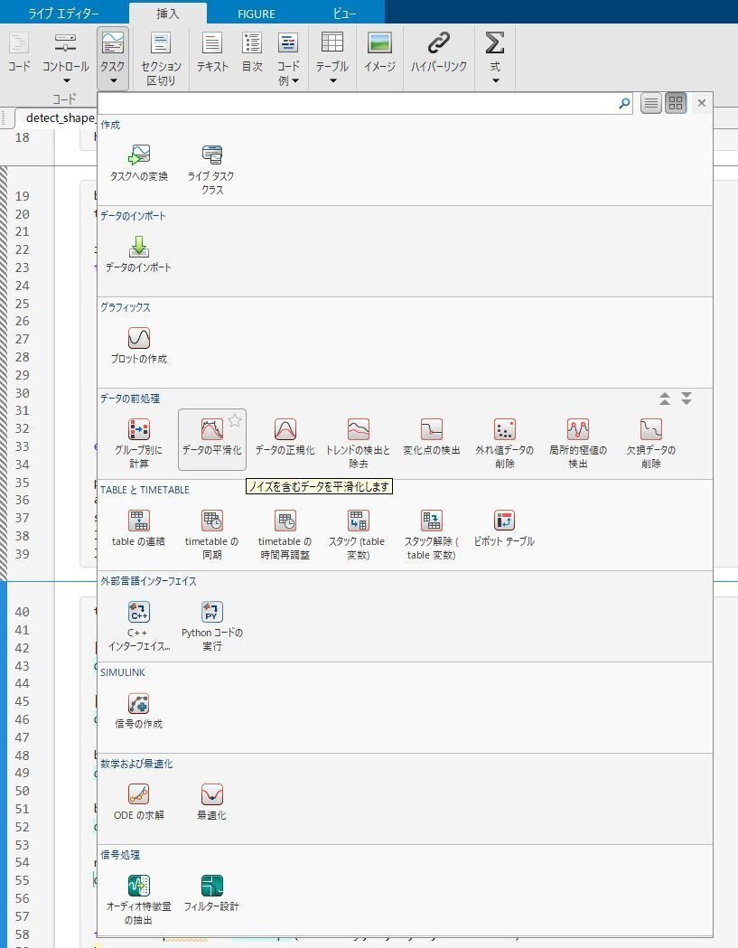
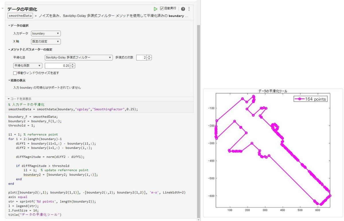
MATLAB には「データの平滑化ツール」が用意されており、コードに挿入するだけで使うことができます。これを利用してもよいでしょう。
穴あき図形
今度はもう少し複雑な図形で試してみましょう。
clear
img = imread('https://blogger.googleusercontent.com/img/b/R29vZ2xl/AVvXsEhqRpXGv-6Jp7IFGPQvO_14GG5nUIJmXNXXvHvYDID8Bh9zr3kXGAQU__z_-mx3LUIab7BVyPdtzrSgfLTNOb0DczNGE-BWY7zmfGkb_Cc4_PQnUo4hX-R-F4va1M_fC2I5uH8WASa0d1uN7ygMpt0EqW9TqpI9EznEFMBt-VIdj-AINRBFzvCtvq3WhgHQ/s180-c/eto_hebi_kamifubuki.png');

imshow(img)

grayImg = rgb2gray(img);
bwImg = imbinarize(grayImg);
[B, L] = bwboundaries(bwImg, CoordinateOrder='xy');

figure
axis equal
hold on
for n = 1:size(B,1)
    boundary = B{n};
    plot(boundary(:,1), -boundary(:,2));
    s(n) = sum(find(L==n)>0);
    fprintf('%3d points\tarea = %d\n', length(boundary), s(n))
end
hold off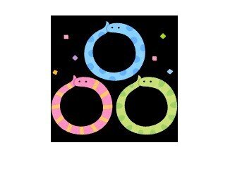
最初に書いたように B にセル形式で各領域の座標データが、L にラベル番号が振られていますので、各領域毎に plot したり、同じラベル番号領域を数えれば面積が分かります。
244 points	area = 2775
 17 points	area = 29
 19 points	area = 31
 16 points	area = 33
243 points	area = 2784
243 points	area = 2789
 20 points	area = 35
 17 points	area = 37
 18 points	area = 37
235 points	area = 2758
  5 points	area = 3
  5 points	area = 4
237 points	area = 2758
  5 points	area = 4
  7 points	area = 5
237 points	area = 2752
  5 points	area = 3
  7 points	area = 5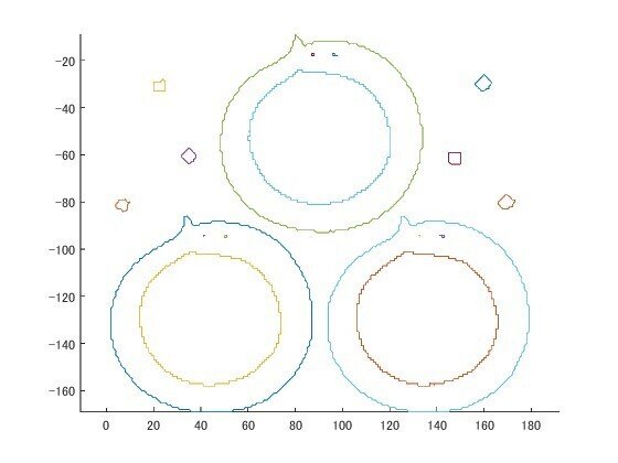
ラベル付けされたデータを個別に表示してみましょう。
figure
tiledlayout('flow','TileSpacing','tight')
for n = 1:size(B,1)
    nexttile
    imshow(L==n)
end
ax = gca;
xl = ax.XLim;  yl = ax.YLim;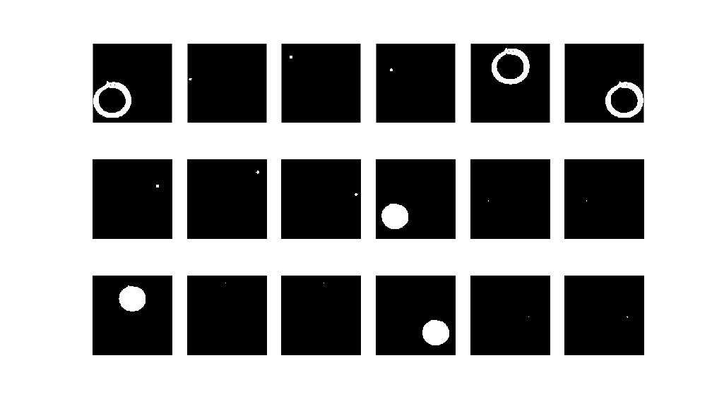
同様に、各境界データも見てみます。
figure
tiledlayout('flow','TileSpacing','tight')
for n = 1:size(B,1)
    nexttile
    boundary = B{n};
    plot(boundary(:,1), -boundary(:,2));
    xlim(xl)
    ylim([-yl(2) -yl(1)])
    axis square
end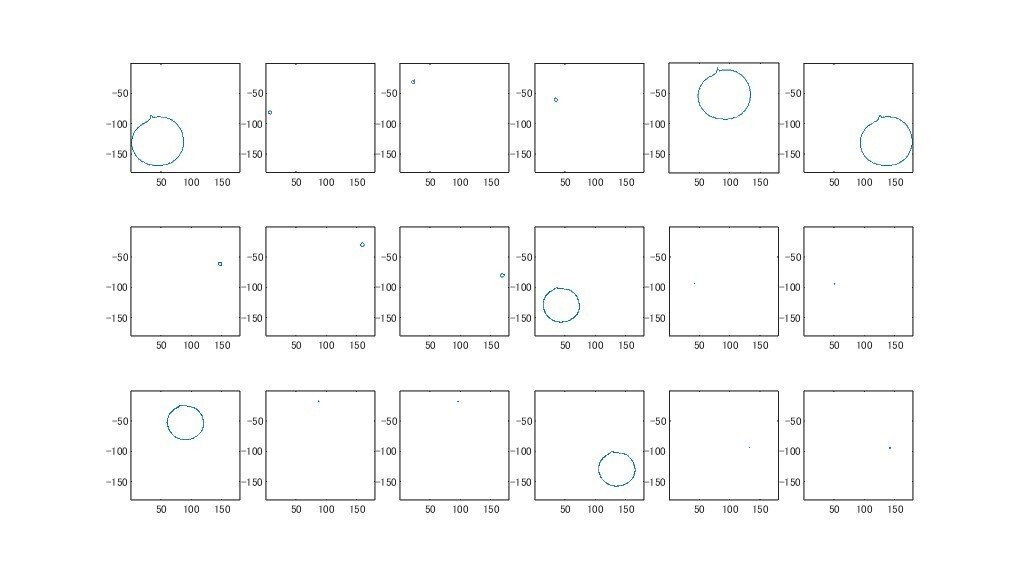
ヘビの目は領域としては小さすぎて後処理で面倒になるので、埋めてしまいましょう。
% 小さな穴の検出とフィルタリング
holes = ~bwImg & imfill(bwImg, 'holes');  % 穴部分だけを抽出
L_holes = bwlabel(holes);  % 穴にラベル付け

% 各穴の面積を計算して小さい穴のみ保持
smallHoleMask = false(size(bwImg));
minHoleSize = 10;  % 小さい穴の最大サイズのしきい値

for k = 1:max(L_holes(:))
    holeArea = sum(L_holes(:) == k);  % 面積を計算
    if holeArea <= minHoleSize
        smallHoleMask = smallHoleMask | (L_holes == k);
    end
end

% 小さな穴を埋める
bwProcessed = bwImg | smallHoleMask;

% 境界の再検出と表示
[B2, L2] = bwboundaries(bwProcessed, CoordinateOrder='xy');

figure
montage({bwImg, holes, smallHoleMask, bwProcessed},"Size",[1 4])

figure
imshow(bwProcessed)
title('Filtered Boundaries without Filling Large Holes');
hold on;

for n = 1:length(B2)
    boundary = B2{n};
    plot(boundary(:,1), boundary(:,2), 'r', 'LineWidth', 1.5);
end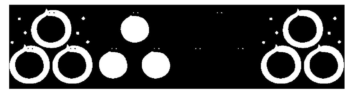
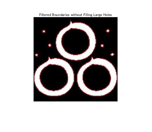
目がなくなると、ヘビとしての面影はなくなるんですね・・。
各ラベリング部分を白にして元画像と重ね合わせるとこんな感じになっています。
figure
tiledlayout('flow','TileSpacing','tight')
for n = idx
    nexttile
    imshow(img + repmat(uint8(L2==n)*250,[1 1 3]))
end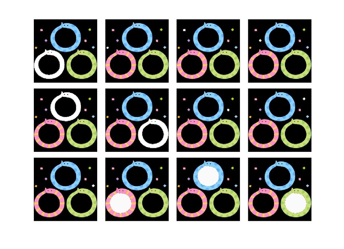
計算幾何学
さて今度は、先ほどとは違った方法でポイントを削減してみましょう。
MATLAB の計算機科学関数である polyshape を使ってみます。
polyshape に関しては、以下の記事もご参照ください。
多角形を一つのオブジェクトとして扱うことができ、幾何学変換・解析等も簡単に行えます。
テキストを見やすい位置に出すために、centroid 関数で領域の重心(ここでは重心のX座標のみ)を用いています。
変換後の座標は、Vertices プロパティで参照できます。
figure
% 境界ごとに polyshape に変換しプロット
warning('off', 'MATLAB:polyshape:repairedBySimplify');
for k = 1:length(B2)
    boundary = B2{k};

    % polyshape オブジェクトの作成
    pgon(k) = polyshape(boundary(:,1), -boundary(:,2));
    p = pgon(k);

    % polyshape の描画
    plot(p, 'FaceAlpha', 0.35);
    hold on

    ar = ceil(area(p));
    text(centroid(p), max(p.Vertices(:,2))-10, string(ar))
    fprintf('%3d points\tarea = %d\n', length(p.Vertices), ar)
end
hold off
axis equal
warning('on', 'MATLAB:polyshape:repairedBySimplify');
title('Boundaries as polyshape Objects');
124 points area = 5418
13 points area = 20
6 points area = 21
9 points area = 25
125 points area = 5429
123 points area = 5427
5 points area = 25
9 points area = 28
12 points area = 28
140 points area = 2640
140 points area = 2639
140 points area = 2633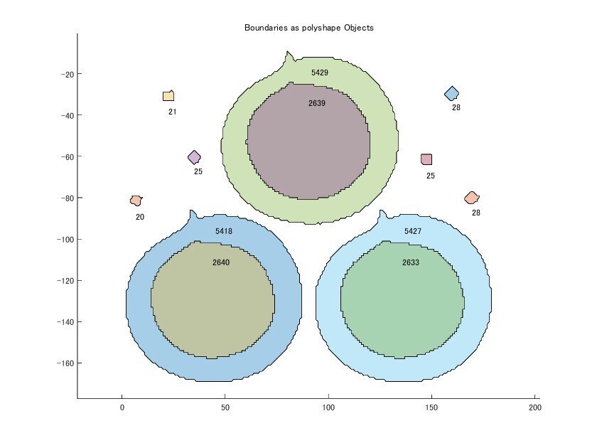
polyshape 関数はデフォルトで自動的に不要なデータ・矛盾データを削除するため、変換するだけでポイント数が減っています。
ただし削減が行われる際に警告が出るため、警告出力を一時的に止めています。
ポイント数の変化を図でも確認しておきましょう。
f = figure;
tiledlayout(1,2)

nexttile
axis square
hold on
for n = 1:length(B2)
    boundary = B2{n};
    plot(boundary(:,1), -boundary(:,2), 'o');
end
hold off

nexttile
axis square
hold on
for n = 1:length(B2)
    p = pgon(n);
    boundary = p.Vertices;
    plot(boundary(:,1), boundary(:,2), 'o');
end
hold off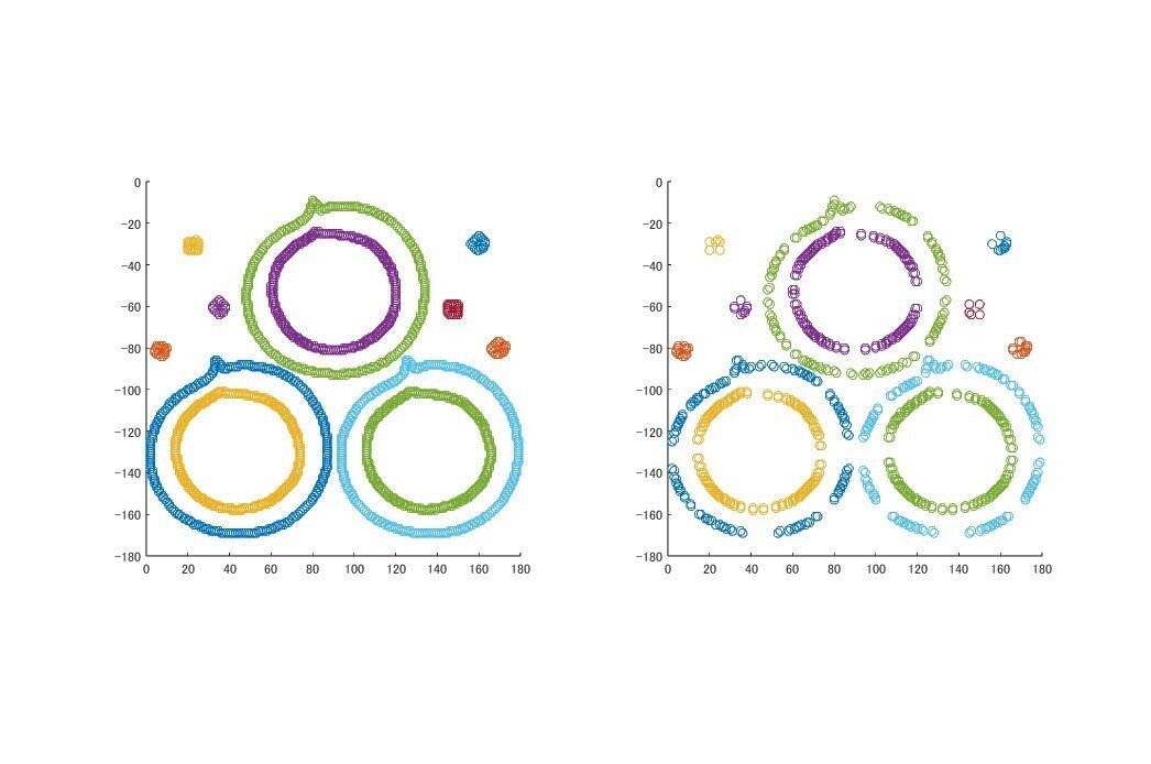
しかし各境界データをそのまま polyshape 化したため「穴」が反映されておらず、各外部領域の面積が増えています。
次は、穴領域を統合しましょう。
内包される穴かどうかは、isinterior 関数で検出できます。
各点が、ある領域の内部にあるかどうかが判定できます。
内包される穴(=全ての点が領域内)であれば、 addboundary 関数で結合します。
f = figure;
% 各ポリゴンについて内包図形を結合
for i = 1:length(pgon)
    % 現在のポリゴンに結合する対象を作成
    currentPolygon = pgon(i);
    for j = 1:length(pgon)
        if i ~= j
            % ポリゴン j がポリゴン i 内部にあるか判定
            if all(isinterior(currentPolygon, pgon(j).Vertices))
                % 内包するポリゴンを結合
                currentPolygon = addboundary(currentPolygon, pgon(j).Vertices);
            end
        end
    end
    % 結合結果の更新
    pgon2(i) = currentPolygon;
end

% 結果の描画

hold on
for k = 1:length(pgon2)
    p = pgon2(k);
    plot(p, 'FaceAlpha', 0.35, 'EdgeColor', 'k');
    ar = ceil(area(p));
    text(centroid(p), max(p.Vertices(:,2))-10, string(ar))
    fprintf('%3d points\tarea = %d\n', length(p.Vertices), ar)
end
title('内包図形の結合結果');
axis equal
265 points area = 2778
13 points area = 20
6 points area = 21
9 points area = 25
266 points area = 2790
264 points area = 2794
5 points area = 25
9 points area = 28
12 points area = 28
140 points area = 2640
140 points area = 2639
140 points area = 2633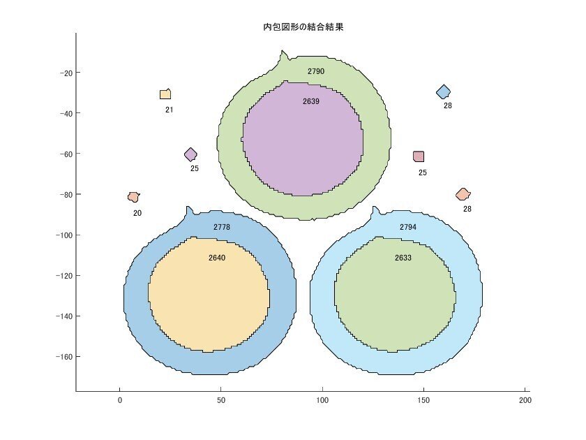
重なっているので分かりにくいですが、外部領域の面積が減っているのが分かるかと思います。
左下領域の結合前後を表示してみましょう。
f = figure;
tiledlayout(1,2)

nexttile
plot(pgon(1))
axis square

nexttile
plot(pgon2(1))
axis square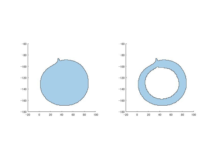
おまけ
ついでに、polyshape 化すると領域単位で幾何学変換等が簡単に行えることを示すために、一領域だけを動かしてみましょう。
拡大・縮小しながら回転させてみます。
見た目の問題で、内包領域結合前のポリゴンを使っています。
各領域、area 関数で面積が得られ、scale、translate、rotate 等の幾何学変換が関数一つで行えます。
% アニメーション1
figure

ph = gobjects(length(pgon), 1);
for k = 1:length(pgon)
    ph(k) = plot(pgon(k), 'FaceAlpha', 0.35);
    hold on;
end
hold off;
ylim([-180 20])
axis equal
axis off

% 最大面積の形状を取得
areas = arrayfun(@(x) area(x), pgon);
[~, idxMax] = max(areas);
maxShape = pgon(idxMax);

% 最大面積の形状の重心を取得
[cx,cy] = centroid(maxShape);

% アニメーションパラメータ
rotationAngles = linspace(0, 360, 100);  % 回転角度 (度)
scaleFactors = 1 - 0.1 * sin(rotationAngles/180*pi*8);  % 収縮率

% アニメーションループ
for i = 1:length(scaleFactors)
    % 形状のスケール
    transformedShape = scale(maxShape, scaleFactors(i));

    % 重心を中心に回転を行う
    transformedShape = rotate(transformedShape, rotationAngles(i), [cx, cy]);

    % 頂点データ更新
    ph(idxMax).Shape.Vertices = transformed2hape.Vertices;

    drawnow
end
もうひとつ、面積の大きい3つを同時に角度を変えてみます。
% アニメーション2
figure

ph = gobjects(length(pgon), 1);
for k = 1:length(pgon)
    ph(k) = plot(pgon(k), 'FaceAlpha', 0.35);
    hold on;
end
hold off;
ylim([-180 20])
xlim([-10 190])
axis square
axis off

% pgon の各 polyshape の面積を計算
areas = arrayfun(@area, pgon);
% 面積の降順でインデックスを取得
[~, sortedIndices] = sort(areas, 'descend');
% 上位3つのインデックスを取得
top3Indices = sortedIndices(1:3);

% アニメーションパラメータ
rotationAngles = repmat([-30 30],1,10); % 回転角度 (度)

gifFileName = "polyMove2.gif";
% アニメーションループ
for i = 1:length(rotationAngles)
    for idx = top3Indices
        [cx,cy] = centroid(pgon(idx));
        % 重心を中心に回転を行う
        transformedShape = rotate(pgon(idx), rotationAngles(i), [cx, cy]);
        % 頂点データ更新
        ph(idx).Shape.Vertices = transformedShape.Vertices;
    end
    drawnow

    % フレームキャプチャ
    frame = getframe(gcf);
    img = frame2im(frame);
    [imind, cm] = rgb2ind(img, 256);
    if i == 1
        imwrite(imind, cm, gifFileName, 'gif', 'Loopcount', inf, 'DelayTime', 0.3);
    else
        imwrite(imind, cm, gifFileName, 'gif', 'WriteMode', 'append', 'DelayTime', 0.3);
    end
    pause(0.3)
end
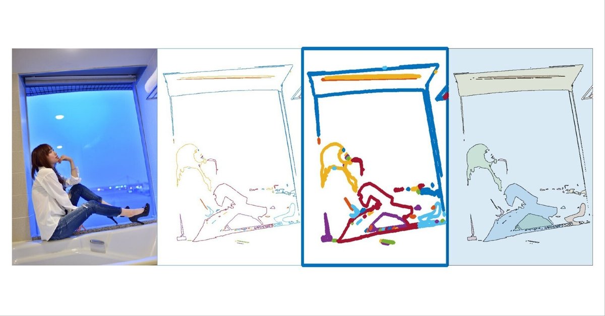
三角形分割とかも triangulation 関数で一発です。
clear

img = imread('ayaka24_0143p.jpg');
img = imresize(img, 0.5);

grayImg = rgb2gray(img);
bwImg = imbinarize(grayImg);
[B, L] = bwboundaries(bwImg, CoordinateOrder='xy');

th = 10;
% 境界ごとに polyshape に変換
warning('off', 'all');
for n = 1:length(B)
    boundary = B{n};
    s(n) = sum(find(L==n)>0);
    if s(n) > th
        % polyshape オブジェクトの作成
        pgon(n) = polyshape(boundary(:,1), -boundary(:,2));
    end
end
warning('on', 'all');

% アニメーション
f = figure;
% f.Position = [100 100 1000 1600];
col = colororder('glow12');
colororder('sail')
colN = size(col,1);

all_vertices = vertcat(pgon.Vertices);
x_min = min(all_vertices(:,1));
x_max = max(all_vertices(:,1));
y_min = min(all_vertices(:,2));
y_max = max(all_vertices(:,2));
f.Position = [100 100 x_max -y_min];
% f.Visible = "on";
% f.Color = [1 1 1];

plot(pgon, 'FaceAlpha', 0.15)
axis equal
axis off
axis([x_min x_max y_min y_max]);
drawnow

gifFileName = "Ayaka_Tri_mov.gif";
frame = getframe(gcf);
img = frame2im(frame);
[imind, cm] = rgb2ind(img, 256);
imwrite(imind, cm, gifFileName, 'gif', 'Loopcount', inf, 'DelayTime', 1);

cn = 1;
for k=1:size(pgon,2)
    p = pgon(k);
    if p.NumRegions > 0
        T = triangulation(p);
        hold on
        triplot(T, Color=col(cn,:))
        cn = mod(cn ,colN) + 1;
        drawnow
        frame = getframe(gcf);
        img = frame2im(frame);
        [imind, cm] = rgb2ind(img, 256);
        imwrite(imind, cm, gifFileName, 'gif', 'WriteMode', 'append', 'DelayTime', 0.1);
    end
end
imwrite(imind, cm, gifFileName, 'gif', 'WriteMode', 'append', 'DelayTime', 1);
hold off
お好みの画像で色を変えたりして試してみてください。
あとがき
やっぱり MATLAB って便利ですね。 (u_u)
テスト画像引用元
タイトル画像モデル:綾夏