
MATLAB R2024b アップデートメモ

まえがき
リリースノート読み、毎回量が多すぎて死にかかってるので、今回は MATLAB 本体に絞って気になったところだけ簡単に。
Audio Toolbox は例のごとくアップデートが少なく、しかも大半が Deep Learning がらみでした。
タイトル画像は、そんな悲しみを表しています。😔
VST の GUI 関連機能アップをぜひ!
Data Analysis
・summary Function
配列の概要を表示する関数です。
これまではカテゴリカル配列のみでしたが、それ以外のデータ型にも対応しました。
>> A = rand(5,3);
>> s = summary(A)

s =

  フィールドをもつ struct:

          Size: [5 3]
          Type: 'double'
    NumMissing: [0 0 0]
           Min: [0.2551 0.1386 0.2435]
        Median: [0.6991 0.2575 0.8143]
           Max: [0.8909 0.9593 0.9293]
          Mean: [0.6205 0.4104 0.6164]
           Std: [0.2465 0.3484 0.3382]
・isbetween Function
区間内の要素を判別する関数です。
これまでは date 型と time 型のみでしたが、それ以外のデータ型にも対応しました。
閉区間・開区間も指定できます。
>> A = 1:9

A =

     1     2     3     4     5     6     7     8     9

>> TF = isbetween(A,3,6)

TF =

  1×9 の logical 配列

   0   0   1   1   1   1   0   0   0

>> TF = isbetween(A,3,6,"open")

TF =

  1×9 の logical 配列

   0   0   0   1   1   0   0   0   0

>> TF = isbetween(A,3,6,"closedleft")

TF =

  1×9 の logical 配列

   0   0   1   1   1   0   0   0   0

>> TF = isbetween(A,3,6,"closedright")

TF =

  1×9 の logical 配列

   0   0   0   1   1   1   0   0   0
・rmmissing and rmoutliers Functions
rmmissing は、欠損値を含むエントリを削除する関数です。
MissingLocations パラメータで削除するインデックスを指定できるようになりました。
これにより、デフォルトの「欠損値(NaN等)」だけでなく、欠損値の条件を設定することができます。
>> A = [1; 4; 9; 12; 3];
B = [9; 0; 6; 2; 1];
C = [14; 4; 2; 3; 8];
>> T = table(A,B,C)

T =

  5×3 table

    A     B    C
    __    _    __

     1    9    14
     4    0     4
     9    6     2
    12    2     3
     3    1     8

>> T = rmmissing(T,MissingLocations=(T>10))

T =

  3×3 table

    A    B    C
    _    _    _

    4    0    4
    9    6    2
    3    1    8
rmoutliers は、外れ値の検出と削除を行う関数です。
既定での外れ値とは、中央値からの距離が中央絶対偏差 (MAD) の 3 倍を超えている値です。
こちらも同様にインデックスによる指定が、OutlierLocations パラメータできるようになりました。
テーブルはライブエディターの方が表示が分かりやすいので、今度はそちらで。

Live Editor
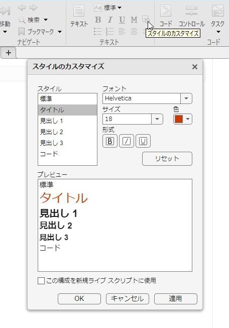
・Customize font styles
フォント・スタイルのカスタマイズができるようになりました。
スタイルのカスタマイズなので、ここで直接テキスト属性を変更できるわけではありません。
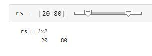
・range sliders
レンジ・スライダーが Live Editor にも追加されました。
・drop-down list
ドロップダウンリストはワークスペースの変数から登録できます。
これまではストリング配列のみ対応でしたが、他のデータ型配列からも可能となりました。

Graphics
・violinplot Function
各カラムごとのデータ分布を表示する violinplot が追加されました。
確かに他で見たことはありますが、使い道がよく分かりません。
こんな使い方しか思いつきませんでした・・。
% rng(0,"twister");  % for reproducibility
ydata = randn(100,3);
v = violinplot(ydata);

numFrames = 30;
axis off
xl = xlim;  yl = ylim;
xlim([xl(1) xl(2)])
ylim([yl(1) yl(2)*10])
r1 = randi(3,1,20);
endFlag = false;
nextFlag = false;
goalLineY = (yl(2) - 1) * 10;
yline(goalLineY, LineWidth=2,Color='b')
for n = r1
    for t = 0:8
        for i = 1:length(v)
            v(n).DensityWidth =  sin(t/numFrames*8*pi)*0.45+0.5;
            v(n).YData = v(n).YData + 0.25;
            if ~endFlag
                if max(v(n).YData) > goalLineY
                    text(n,max(v(n).YData)+5,'Win!!', ...
                        FontSize=14,Color='r',FontWeight='bold')
                    endFlag = true;
                    win = n;
                end
            else
                if max(v(n).YData) > goalLineY
                    if (win ~= n)
                        if ~nextFlag
                            col = v(n).EdgeColor;
                        else
                            col = col * 0.98;
                        end

                        text(n,max(v(n).YData)+5,'No!!', ...
                            FontSize=14,Color=col,FontWeight='bold')
                        nextFlag = true;
                    end
                end
            end
        end
        drawnow;
    end
end
if ~endFlag
    text(1,0,'Time Up!', ...
        FontSize=14,Color='r',FontWeight='bold')
end
「正しい使い方」をご存じの方がいらっしゃれば教えてください。
・compassplot Function
原点からの矢印を描く関数です。
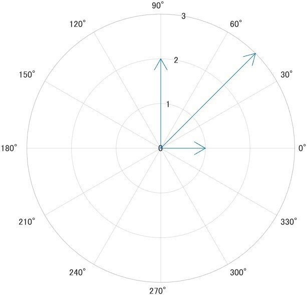
元々類似機能の compass 関数がありましたが、よりプロパティの多いcompssplot への置き換えが推奨されています。
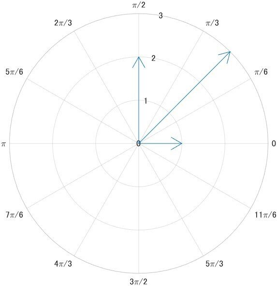
極座標の角度単位もプロパティで切り替えられます。
theta = [0 pi/4 pi/2]';
rho = [1 3 2]';
t = table(theta,rho);
compassplot(t,"theta","rho")

pax = gca;
exportgraphics(pax,'compassplot_deg.jpg')
pax.ThetaAxisUnits = "radians";
exportgraphics(pax,'compassplot_rad.jpg')
・constantplane Function
3D グラフで、範囲指定不要なプレーンを描画します。
normal=[a b c]、offset=d のとき、constantplane(normal, offset) で
ax + by + cz = d のプレーンが描画されます。
x/y/z 各コンスタント・プレーンは、オフセット指定のみで簡単に描くことができます。
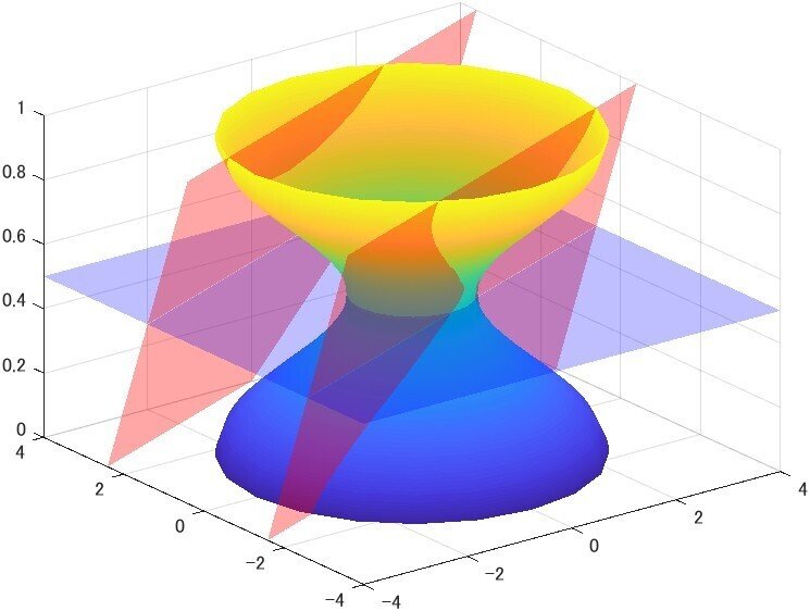
t = 0:pi/20:2*pi;
r = 2 + cos(t);
[X,Y,Z] = cylinder(r);
s = surf(X,Y,Z);
s.EdgeColor = "none";

normal = [-0.2 0.5 1; -0.2 0.5 1];
offset = [0 2];
constantplane(normal, offset, FaceColor = "r", FaceAlpha=0.35);
constantplane("z", 0.5, FaceColor = "b", FaceAlpha=0.25);
xlim([-4 4])
ylim([-4 4])
・Legends
凡例のアイコン部分の幅を変えられるようになりました。
単位は point (1/72 inch)です。
これはなにげに欲しかった機能ですね!

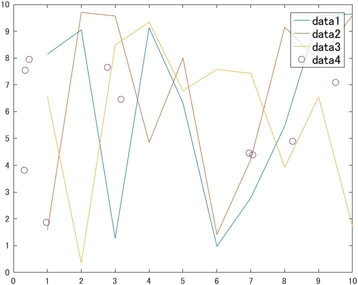
rng default
p = plot(rand(10,3)*10);
hold on
scatter(rand(10,1)*10,rand(10,1)*10)
hold off
l = legend;
l.FontSize = 12;
l.BackgroundAlpha = 0.75;
ax = gca;
exportgraphics(ax,'Legend_def.jpg')
l.IconColumnWidth = 15;
exportgraphics(ax,'Legend_15.jpg')
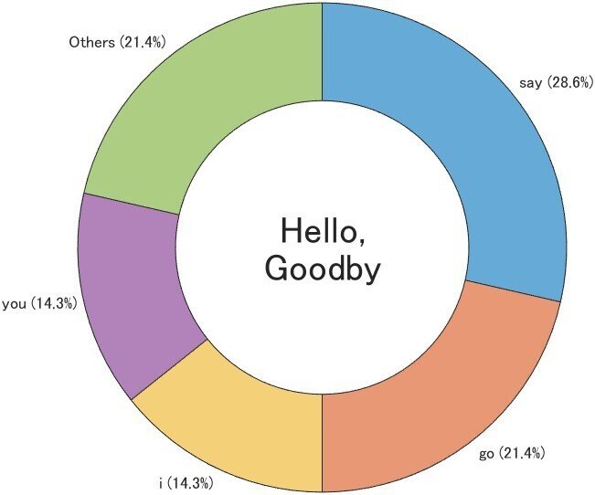
l.IconColumnWidthMode = "auto";・Pie Charts and Donut Charts
piechart / donutchart で、表示スライス数が設定できるようになりました。
残りはまとめて "Others" で表示されます。表示を逆順にすることも、"Others" を表示しないこともできます。
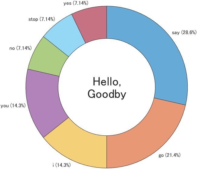
str = "You say yes, I say no, You say stop and I say go go go.";

% split words
pat = " " | "," | "." | "and";
words = split(str,pat);
words = lower(words);
words(words == "") = [];

[w,~,idx] = unique(words);
hNum = histcounts(idx,numel(w));
[hNumSorted,idx2] = sort(hNum,'descend');
wSorted = w(idx2);

w2 = categorical(words);
rank2 = reordercats(w2,wSorted);
d = donutchart(rank2);

d.CenterLabel = ["Hello," "Goodby"];
d.CenterLabelFontSize = 20;

ax = gca;
exportgraphics(ax,'DonutChart1.jpg')

d.NumDisplayWedges = 4;
exportgraphics(ax,'DonutChart2.jpg')
・Bar Charts
バー自体にラベルを付けられるようになりました。位置も外側か内側か指定できます。
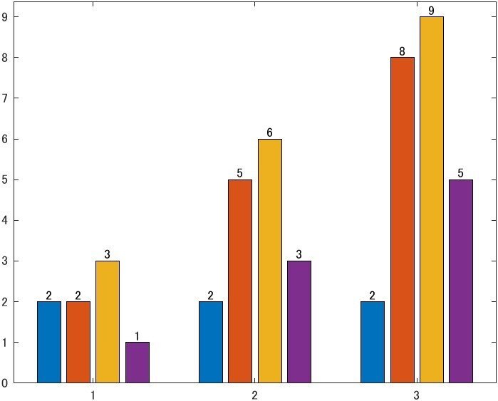
barData = [2 2 3 1; 2 5 6 3; 2 8 9 5];
b = bar(barData);
set(b,{"Labels"},num2cell(barData,1)')
ax = gca;
exportgraphics(ax,'barLabel1.jpg')
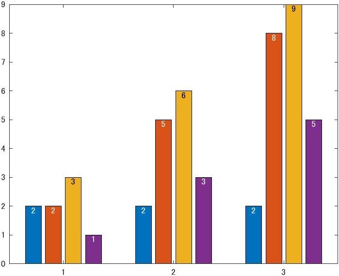
set(b,"LabelLocation","end-inside")
exportgraphics(ax,'barLabel2.jpg')
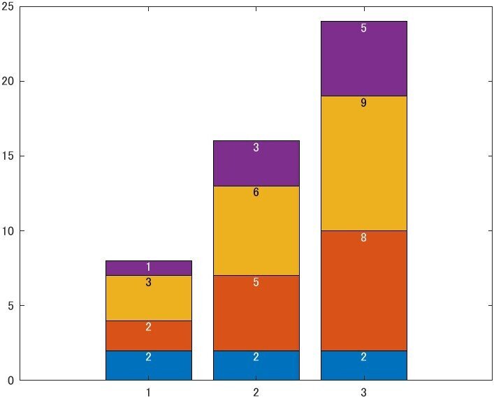
set(b,"BarLayout","stacked")
exportgraphics(ax,'barLabel3.jpg')
個別に指定するにはその列を指定します。列毎(このグラフでは同じ色毎)にしか指定はできません。(grouped/stacked はグラフ毎)

set(b,"BarLayout","grouped")
b(end).LabelLocation = "end-outside";
・ConstantLine Object
xline/yline のラベルの色が、ラインと別に設定できるようになりました。
今まではラインの色と同色になっていました。

plot([0 1; 1 2; 2 3; 3 4; 4 5; 5 6])
xregion(2,3,FaceAlpha=1,FaceColor=[0.6 0.7 0.9])
yl = yline(3);
xr = xregion([4 5],FaceAlpha=1,FaceColor=[0.95 0.7 0.6],Layer="top");

yl.Label = "\mu";
yl.LineStyle = "--";
yl.FontSize = 18;
yl.Interpreter = "tex";
yl.Color = "m";
yl.LabelColor = "g";
App Building
・uibutton and uitogglebutton Functions
ボタンやトグルボタンでも、テキスト・インタープリターが使えるようになりました。html や latex が指定できます。
R2024a で、ラジオボタンでは使えるようになっていました。

fig = uifigure('Position',[300 300 400 450]);

% R2024a later
p1 = uipanel(fig, "Title","R2024a later", Position = [50 25 300 200]);
bg = uibuttongroup(p1,'Position',[0 0 300 200-20]);
rb1 = uiradiobutton(bg,'Position',[10 120 250 40],"Interpreter","latex");
rb2 = uiradiobutton(bg,'Position',[10 70 100 40]);
rb3 = uiradiobutton(bg,'Position',[10 20 100 40]);

rb1.Text = '$F(\omega) = \int_{-\infty}^{\infty} f(t) e^{-j\omega t} dt$';
rb1.FontSize = 18;
rb2.Interpreter = "html";
rb2.Text = '<p style="color: red;">html</p>';
rb3.Text = 'Text';
rb3.FontColor = "#f04080";


% New in R2024b
p2 = uipanel(fig, "Title","New in R2024b", BackgroundColor = 'w', Position = [50 225 300 200]);
bg2 = uibuttongroup(p2,'Position',[0 0 300 200-20], BackgroundColor = 'w');
ub = uibutton(bg2,'Position',[10 120 200 50],Interpreter="latex", Icon="info");
ub.Text = '$$\int_{-\infty} ^\infty x^2 dx$$';
sb = uibutton(bg2,'state','Position',[10 60 200 50],"Interpreter","latex", Icon="success");
sb.Text = '$$F(\omega) = \int_{-\infty}^{\infty} f(t) e^{-j\omega t} dt$$';
あとがき
ほんといつも、ワクワクもしますがざっと見るだけでも大変です。
秋の夜長、MATLAB リリース ノート を眺めて過ごしてみてはいかがでしょうか。(u_u)
タイトル画像モデル:凛