
第10章:ベイジアンML-ダイナミックSR 第5節: 確率的ボラティリティモデル

インポートと設定
import warnings
warnings.filterwarnings('ignore')
%matplotlib inline
from pathlib import Path
import numpy as np
import pandas as pd
import matplotlib.pyplot as plt
from matplotlib.ticker import FuncFormatter
import seaborn as sns
import pymc3 as pm
from pymc3.distributions.timeseries import GaussianRandomWalksns.set_style('whitegrid')
# model_path = Path('models')モデルの仮定
資産価格は時変ボラティリティ(日ごとの収益の変動)を持っています。一部の期間では、株価は非常に変動しやすく、他の期間では非常に安定しています。確率的ボラティリティモデルは、潜在的ボラティリティ変数を使用してこれをモデル化し、確率過程としてモデル化します。
次のモデルは、No-U-Turn Samplerの論文、Hoffman(2011)p21で説明されているモデルに似ています。
σ~Exponential(50)
v~Exponential(0.1)
s_i ~ Normal(s_{i-1}, σ^{-2})
log(r_i) ~ t(v, 0, exp(-2s_i))
ただし、rは日次リターンでsは潜在的ログボラティリティ過程
価格データの取得
今回はS&P 500を使います。
prices = pd.read_hdf('../data/assets.h5', key='sp500/stooq').loc['2000':, 'close']
log_returns = np.log(prices).diff().dropna()
ax = log_returns.plot(figsize=(15, 4),
title='S&P 500 | Daily Log Returns',
rot=0)
ax.yaxis.set_major_formatter(FuncFormatter(lambda y, _: '{:.0%}'.format(y)))
sns.despine()
plt.tight_layout();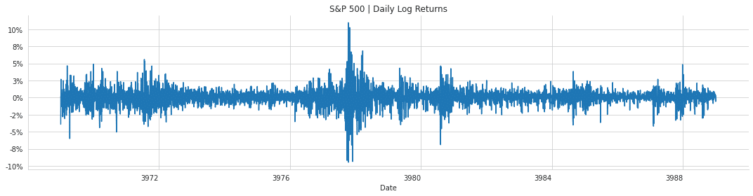
PyMC3でモデルを特定する。
with pm.Model() as model:
   step_size = pm.Exponential('sigma', 50.)
   s = GaussianRandomWalk('s', sd=step_size,
                          shape=len(log_returns))
   nu = pm.Exponential('nu', .1)
   r = pm.StudentT('r', nu=nu,
                   lam=pm.math.exp(-2*s),
observed=log_returns)pm.model_to_graphviz(model)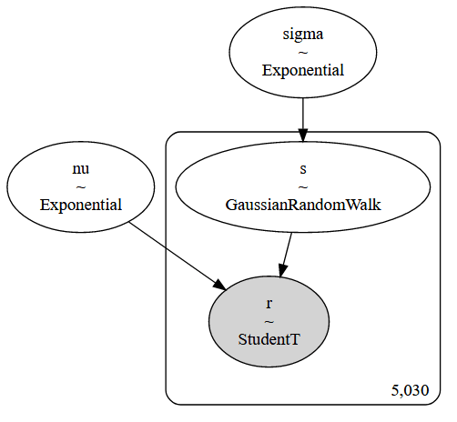
モデルのフィッティング
with model:
   trace = pm.sample(tune=2000,
                     draws=5000,
                     chains=4,
                     cores=1,
                     target_accept=.9)
結果の評価
痕跡プロット
pm.traceplot(trace, varnames=['sigma', 'nu']);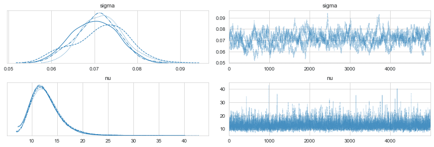
インサンプル予測
pm.trace_to_dataframe(trace).info()
'''
<class 'pandas.core.frame.DataFrame'>
RangeIndex: 4000 entries, 0 to 3999
Columns: 5032 entries, s__0 to nu
dtypes: float64(5032)
memory usage: 153.6 MB
'''
fig, ax = plt.subplots(figsize=(15, 5))
log_returns.plot(ax=ax, lw=.5, xlim=('2000', '2020'), rot=0,
title='In-Sample Fit of Stochastic Volatility Model')
ax.plot(log_returns.index, np.exp(trace[s]).T, 'r', alpha=.03, lw=.5);
ax.set(xlabel='Time', ylabel='Returns')
ax.legend(['S&P 500 (log returns)', 'Stochastic Volatility Model'])
ax.yaxis.set_major_formatter(FuncFormatter(lambda y, _: '{:.0%}'.format(y)))
sns.despine()
fig.tight_layout();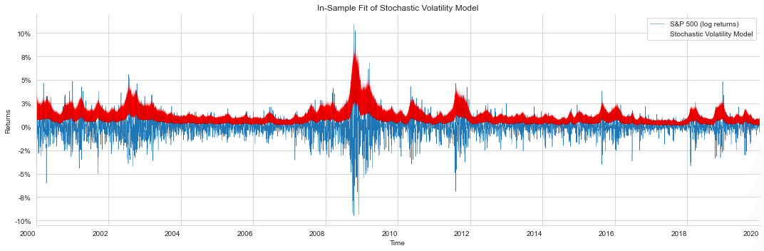
この記事が気に入ったらサポートをしてみませんか?