
第9章 ボラティリティ予測と統計的裁定取引 第6節: 共和分検定とカルマンフィルターを利用したペアトレーディング

この記事では、タイトルの通り、共和分検定とカルマンフィルターを用いてペアトレーディング出来るような資産を見つけることが目的です。
仮想通貨であれば、アルトコイン同士でペアトレーディングするのも中々面白そうではありますよね。
インポートと設定
import warnings
warnings.filterwarnings('ignore')
from collections import Counter
from time import time
from pathlib import Path
import numpy as np
import pandas as pd
from pykalman import KalmanFilter
from statsmodels.tsa.stattools import coint
from statsmodels.tsa.vector_ar.vecm import coint_johansen
from statsmodels.tsa.api import VAR
import matplotlib.pyplot as plt
import seaborn as snsidx = pd.IndexSlice
sns.set_style('whitegrid')def format_time(t):
m_, s = divmod(t, 60)
h, m = divmod(m_, 60)
return f'{h:>02.0f}:{m:>02.0f}:{s:>02.0f}'ヨハンセン検定 異常値定義
critical_values = {0: {.9: 13.4294, .95: 15.4943, .99: 19.9349},
                  1: {.9: 2.7055, .95: 3.8415, .99: 6.6349}}
trace0_cv = critical_values[0][.95] # critical value for 0 cointegration relationships
trace1_cv = critical_values[1][.95] # critical value for 1 cointegration relationshipデータの読み込み
DATA_PATH = Path('..', 'data')
STORE = DATA_PATH / 'assets.h5'
バックテスト用の価格取得
関連株とETFのOHLCVデータを結合
def get_backtest_prices():
   with pd.HDFStore('data.h5') as store:
       tickers = store['tickers']

   with pd.HDFStore(STORE) as store:
       prices = (pd.concat([
           store['stooq/us/nyse/stocks/prices'],
           store['stooq/us/nyse/etfs/prices'],
           store['stooq/us/nasdaq/etfs/prices'],
           store['stooq/us/nasdaq/stocks/prices']])
                 .sort_index()
                 .loc[idx[tickers.index, '2016':'2019'], :])
   print(prices.info(null_counts=True))
   prices.to_hdf('backtest.h5', 'prices')
   tickers.to_hdf('backtest.h5', 'tickers')
get_backtest_prices()
'''
<class 'pandas.core.frame.DataFrame'>
MultiIndex: 313869 entries, ('AA.US', Timestamp('2016-01-04 00:00:00')) to ('YUM.US', Timestamp('2019-12-31 00:00:00'))
Data columns (total 5 columns):
# Column Non-Null Count Dtype
--- ------ -------------- -----
0 open 313869 non-null float64
1 high 313869 non-null float64
2 low 313869 non-null float64
3 close 313869 non-null float64
4 volume 313869 non-null int64
dtypes: float64(4), int64(1)
memory usage: 13.3+ MB
None
'''株価の読み込み
stocks = pd.read_hdf('data.h5', 'stocks/close').loc['2015':]
stocks.info()
'''
<class 'pandas.core.frame.DataFrame'>
DatetimeIndex: 1258 entries, 2015-01-02 to 2019-12-31
Columns: 173 entries, AA.US to YUM.US
dtypes: float64(173)
memory usage: 1.7 MB
'''
ETFデータの読み込み
etfs = pd.read_hdf('data.h5', 'etfs/close').loc['2015':]
etfs.info()
'''
<class 'pandas.core.frame.DataFrame'>
DatetimeIndex: 1258 entries, 2015-01-02 to 2019-12-31
Columns: 139 entries, AAXJ.US to YCS.US
dtypes: float64(139)
memory usage: 1.3 MB
'''
ティッカー辞書の読み込み
names = pd.read_hdf('data.h5', 'tickers').to_dict()pd.Series(names).count()
'''
312
'''共和分検定の計算準備
def test_cointegration(etfs, stocks, test_end, lookback=2):
   start = time()
   results = []
   test_start = test_end - pd.DateOffset(years=lookback) + pd.DateOffset(days=1)
   etf_tickers = etfs.columns.tolist()
   etf_data = etfs.loc[str(test_start):str(test_end)]

   stock_tickers = stocks.columns.tolist()
   stock_data = stocks.loc[str(test_start):str(test_end)]
   n = len(etf_tickers) * len(stock_tickers)
   j = 0
   for i, s1 in enumerate(etf_tickers, 1):
       for s2 in stock_tickers:
           j += 1
           if j % 1000 == 0:
               print(f'\t{j:5,.0f} ({j/n:3.1%}) | {time() - start:.2f}')
           df = etf_data.loc[:, [s1]].dropna().join(stock_data.loc[:, [s2]].dropna(), how='inner')
           with warnings.catch_warnings():
               warnings.simplefilter('ignore')
               var = VAR(df)
               lags = var.select_order()
               result = [test_end, s1, s2]
               order = lags.selected_orders['aic']
               result += [coint(df[s1], df[s2], trend='c')[1], coint(df[s2], df[s1], trend='c')[1]]

           cj = coint_johansen(df, det_order=0, k_ar_diff=order)
           result += (list(cj.lr1) + list(cj.lr2) + list(cj.evec[:, cj.ind[0]]))
           results.append(result)
   return results
テスト期間の設定
dates = stocks.loc['2016-12':'2019-6'].resample('Q').last().index検定の実行
ここは恐ろしく時間がかかるので、少ない銘柄で試すことをお勧めします。
test_results = []
columns = ['test_end', 's1', 's2', 'eg1', 'eg2',
          'trace0', 'trace1', 'eig0', 'eig1', 'w1', 'w2']

for test_end in dates:
   print(test_end)
   result = test_cointegration(etfs, stocks, test_end=test_end)
   test_results.append(pd.DataFrame(result, columns=columns))

pd.concat(test_results).to_hdf('backtest.h5', 'cointegration_test')
検定結果の読み込み
test_results = pd.read_hdf('backtest.h5', 'cointegration_test')
test_results.info()
'''
<class 'pandas.core.frame.DataFrame'>
Int64Index: 264517 entries, 0 to 24046
Data columns (total 11 columns):
#   Column    Non-Null Count   Dtype
---  ------    --------------   -----
0   test_end  264517 non-null  datetime64[ns]
1   s1        264517 non-null  object
2   s2        264517 non-null  object
3   eg1       264517 non-null  float64
4   eg2       264517 non-null  float64
5   trace0    264517 non-null  float64
6   trace1    264517 non-null  float64
7   eig0      264517 non-null  float64
8   eig1      264517 non-null  float64
9   w1        264517 non-null  float64
10  w2        264517 non-null  float64
dtypes: datetime64[ns](1), float64(8), object(2)
memory usage: 24.2+ MB
'''
共和分ペアを見つける
ヨハンセン検定
test_results['joh_sig'] = ((test_results.trace0 > trace0_cv) &
(test_results.trace1 > trace1_cv))test_results.joh_sig.value_counts(normalize=True)
'''
False 0.947406
True 0.052594
Name: joh_sig, dtype: float64
'''大体5%くらいはヒットしています。
Engle Granger検定
test_results['eg'] = test_results[['eg1', 'eg2']].min(axis=1)
test_results['s1_dep'] = test_results.eg1 < test_results.eg2
test_results['eg_sig'] = (test_results.eg < .05)test_results.eg_sig.value_counts(normalize=True)
'''
False 0.91128
True 0.08872
Name: eg_sig, dtype: float64
'''Engle-Granger vs Johansen 比較
ここでは両方の検定でどちらにも引っ掛かったものを取得します。
test_results['coint'] = (test_results.eg_sig & test_results.joh_sig)
test_results.coint.value_counts(normalize=True)
'''
False    0.986829
True     0.013171
Name: coint, dtype: float64
'''
test_results = test_results.drop(['eg1', 'eg2', 'trace0', 'trace1', 'eig0', 'eig1'], axis=1)
test_results.info()
'''
<class 'pandas.core.frame.DataFrame'>
Int64Index: 264517 entries, 0 to 24046
Data columns (total 10 columns):
# Column Non-Null Count Dtype
--- ------ -------------- -----
0 test_end 264517 non-null datetime64[ns]
1 s1 264517 non-null object
2 s2 264517 non-null object
3 w1 264517 non-null float64
4 w2 264517 non-null float64
5 joh_sig 264517 non-null bool
6 eg 264517 non-null float64
7 s1_dep 264517 non-null bool
8 eg_sig 264517 non-null bool
9 coint 264517 non-null bool
dtypes: bool(4), datetime64[ns](1), float64(3), object(2)
memory usage: 15.1+ MB
'''ペア数の推移
ax = test_results.groupby('test_end').coint.mean().to_frame('# Pairs').plot()
ax.axhline(.05, lw=1, ls='--', c='k');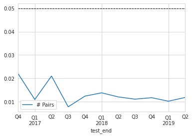
候補ペアの選定
def select_candidate_pairs(data):
   candidates = data[data.joh_sig | data.eg_sig]
   candidates['y'] = candidates.apply(lambda x: x.s1 if x.s1_dep else x.s2, axis=1)
   candidates['x'] = candidates.apply(lambda x: x.s2 if x.s1_dep else x.s1, axis=1)
   return candidates.drop(['s1_dep', 's1', 's2'], axis=1)
candidates = select_candidate_pairs(test_results)candidates.to_hdf('backtest.h5', 'candidates')candidates = pd.read_hdf('backtest.h5', 'candidates')
candidates.info()
'''
<class 'pandas.core.frame.DataFrame'>
Int64Index: 33896 entries, 7 to 24045
Data columns (total 9 columns):
# Column Non-Null Count Dtype
--- ------ -------------- -----
0 test_end 33896 non-null datetime64[ns]
1 w1 33896 non-null float64
2 w2 33896 non-null float64
3 joh_sig 33896 non-null bool
4 eg 33896 non-null float64
5 eg_sig 33896 non-null bool
6 coint 33896 non-null bool
7 y 33896 non-null object
8 x 33896 non-null object
dtypes: bool(3), datetime64[ns](1), float64(3), object(2)
memory usage: 1.9+ MB
'''候補数の推移
candidates.groupby('test_end').size().plot(figsize=(8, 5))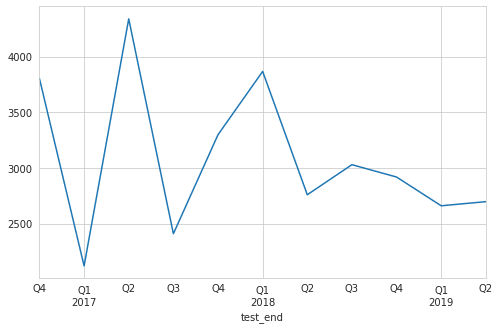
最も共通点が多いペア
時刻によって異常と見なされたペアが異なるので、ここでは、検定に引っ掛かったペアをひたすらカウントして、最もカウントに引っ掛かったペアを出力します。
with pd.HDFStore('data.h5') as store:
   print(store.info())
   tickers = store['tickers']
'''
<class 'pandas.io.pytables.HDFStore'>
File path: data.h5
/etfs/close              frame        (shape->[2516,139])
/stocks/close            frame        (shape->[2516,173])
/tickers                 series       (shape->[1])
'''
with pd.HDFStore('backtest.h5') as store:
print(store.info())
'''
<class 'pandas.io.pytables.HDFStore'>
File path: backtest.h5
/candidates frame (shape->[33896,9])
/cointegration_test frame (shape->[264517,11])
/half_lives frame (shape->[33896,4])
/pair_data frame (shape->[4259004,7])
/pair_trades frame (shape->[1,6])
/prices frame (shape->[313869,5])
/tickers series (shape->[1])
'''counter = Counter()
for s1, s2 in zip(candidates[candidates.joh_sig & candidates.eg_sig].y,
candidates[candidates.joh_sig & candidates.eg_sig].x):
if s1 > s2:
counter[(s2, s1)] += 1
else:
counter[(s1, s2)] += 1most_common_pairs = pd.DataFrame(counter.most_common(10))
most_common_pairs = pd.DataFrame(most_common_pairs[0].values.tolist(), columns=['s1', 's2'])
most_common_pairs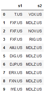
ペアトレの候補が出てきましたね(*'ω'*)
with pd.HDFStore('backtest.h5') as store:
   prices = store['prices'].close.unstack('ticker').ffill(limit=5)
   tickers = store['tickers'].to_dict()
cnt = pd.Series(counter).reset_index()
cnt.columns = ['s1', 's2', 'n']
cnt['name1'] = cnt.s1.map(tickers)
cnt['name2'] = cnt.s2.map(tickers)
cnt.nlargest(10, columns='n')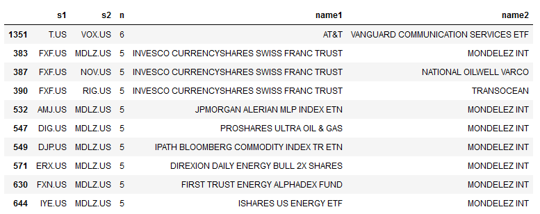
炙り出された似ているペアを確認
fig, axes = plt.subplots(ncols=2, figsize=(14, 5))
for i in [0, 1]:
   s1, s2 = most_common_pairs.at[i, 's1'], most_common_pairs.at[i, 's2']
   prices.loc[:, [s1, s2]].rename(columns=tickers).plot(secondary_y=tickers[s2],
                                                        ax=axes[i],
                                                        rot=0)
   axes[i].grid(False)
   axes[i].set_xlabel('')

sns.despine()
fig.tight_layout()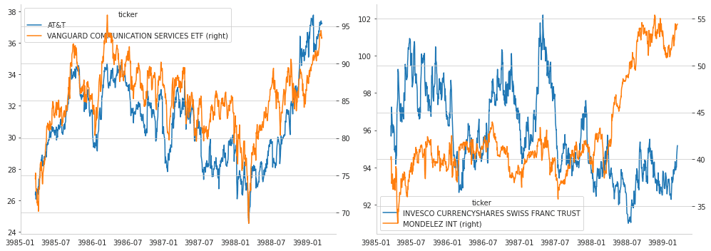
さて、ペアが見つかったら、いよいよ、トレーディング戦略の方に移ります。
カルマンフィルターによるスムージング
def KFSmoother(prices):
   """Estimate rolling mean"""

   kf = KalmanFilter(transition_matrices=np.eye(1),
                     observation_matrices=np.eye(1),
                     initial_state_mean=0,
                     initial_state_covariance=1,
                     observation_covariance=1,
                     transition_covariance=.05)

   state_means, _ = kf.filter(prices.values)
   return pd.Series(state_means.flatten(),
                    index=prices.index)
smoothed_prices = prices.apply(KFSmoother)
smoothed_prices.to_hdf('tmp.h5', 'smoothed')smoothed_prices = pd.read_hdf('tmp.h5', 'smoothed')ローリングヘッジレシオをカルマンフィルターを用いて計算する
def KFHedgeRatio(x, y):
   """Estimate Hedge Ratio"""
   delta = 1e-3
   trans_cov = delta / (1 - delta) * np.eye(2)
   obs_mat = np.expand_dims(np.vstack([[x], [np.ones(len(x))]]).T, axis=1)

   kf = KalmanFilter(n_dim_obs=1, n_dim_state=2,
                     initial_state_mean=[0, 0],
                     initial_state_covariance=np.ones((2, 2)),
                     transition_matrices=np.eye(2),
                     observation_matrices=obs_mat,
                     observation_covariance=2,
                     transition_covariance=trans_cov)

   state_means, _ = kf.filter(y.values)
   return -state_means
平均回帰半減期の推定
def estimate_half_life(spread):
   X = spread.shift().iloc[1:].to_frame().assign(const=1)
   y = spread.diff().iloc[1:]
   beta = (np.linalg.inv(X.T @ X) @ X.T @ y).iloc[0]
   halflife = int(round(-np.log(2) / beta, 0))
   return max(halflife, 1)
スプレッドとボリンジャーバンドの計算
def get_spread(candidates, prices):
   pairs = []
   half_lives = []

   periods = pd.DatetimeIndex(sorted(candidates.test_end.unique()))
   start = time()
   for p, test_end in enumerate(periods, 1):
       start_iteration = time()

       period_candidates = candidates.loc[candidates.test_end == test_end, ['y', 'x']]
       trading_start = test_end + pd.DateOffset(days=1)
       t = trading_start - pd.DateOffset(years=2)
       T = trading_start + pd.DateOffset(months=6) - pd.DateOffset(days=1)
       max_window = len(prices.loc[t: test_end].index)
       print(test_end.date(), len(period_candidates))
       for i, (y, x) in enumerate(zip(period_candidates.y, period_candidates.x), 1):
           if i % 1000 == 0:
               msg = f'{i:5.0f} | {time() - start_iteration:7.1f} | {time() - start:10.1f}'
               print(msg)
           pair = prices.loc[t: T, [y, x]]
           pair['hedge_ratio'] = KFHedgeRatio(y=KFSmoother(prices.loc[t: T, y]),
                                              x=KFSmoother(prices.loc[t: T, x]))[:, 0]
           pair['spread'] = pair[y].add(pair[x].mul(pair.hedge_ratio))
           half_life = estimate_half_life(pair.spread.loc[t: test_end])

           spread = pair.spread.rolling(window=min(2 * half_life, max_window))
           pair['z_score'] = pair.spread.sub(spread.mean()).div(spread.std())
           pairs.append(pair.loc[trading_start: T].assign(s1=y, s2=x, period=p, pair=i).drop([x, y], axis=1))

           half_lives.append([test_end, y, x, half_life])
   return pairs, half_lives
candidates = pd.read_hdf('backtest.h5', 'candidates')
candidates.info()
'''
<class 'pandas.core.frame.DataFrame'>
Int64Index: 33896 entries, 7 to 24045
Data columns (total 9 columns):
# Column Non-Null Count Dtype
--- ------ -------------- -----
0 test_end 33896 non-null datetime64[ns]
1 w1 33896 non-null float64
2 w2 33896 non-null float64
3 joh_sig 33896 non-null bool
4 eg 33896 non-null float64
5 eg_sig 33896 non-null bool
6 coint 33896 non-null bool
7 y 33896 non-null object
8 x 33896 non-null object
dtypes: bool(3), datetime64[ns](1), float64(3), object(2)
memory usage: 1.9+ MB
'''pairs, half_lives = get_spread(candidates, smoothed_prices)結果集計
半減期
hl = pd.DataFrame(half_lives, columns=['test_end', 's1', 's2', 'half_life'])
hl.info()
'''
<class 'pandas.core.frame.DataFrame'>
RangeIndex: 33896 entries, 0 to 33895
Data columns (total 4 columns):
#   Column     Non-Null Count  Dtype
---  ------     --------------  -----
0   test_end   33896 non-null  datetime64[ns]
1   s1         33896 non-null  object
2   s2         33896 non-null  object
3   half_life  33896 non-null  int64
dtypes: datetime64[ns](1), int64(1), object(2)
memory usage: 1.0+ MB
'''
hl.half_life.describe()
'''
count 33896.000000
mean 25.167837
std 10.235579
min 1.000000
25% 20.000000
50% 24.000000
75% 28.000000
max 1057.000000
Name: half_life, dtype: float64
'''hl.to_hdf('backtest.h5', 'half_lives')ペアデータ
pair_data = pd.concat(pairs)
pair_data.info(null_counts=True)
'''
pair_data = pd.concat(pairs)

pair_data.info(null_counts=True)

<class 'pandas.core.frame.DataFrame'>
DatetimeIndex: 4259004 entries, 2017-01-03 to 2019-12-31
Data columns (total 7 columns):
#   Column       Non-Null Count    Dtype
---  ------       --------------    -----
0   hedge_ratio  4259004 non-null  float64
1   spread       4259004 non-null  float64
2   z_score      4259004 non-null  float64
3   s1           4259004 non-null  object
4   s2           4259004 non-null  object
5   period       4259004 non-null  int64
6   pair         4259004 non-null  int64
dtypes: float64(3), int64(2), object(2)
memory usage: 259.9+ MB
'''pair_data.to_hdf('backtest.h5', 'pair_data')pair_data = pd.read_hdf('backtest.h5', 'pair_data')ロングショートのエントリーとエグジットの日付を見つける
def get_trades(data):
   pair_trades = []
   for i, ((period, s1, s2), pair) in enumerate(data.groupby(['period', 's1', 's2']), 1):
       if i % 100 == 0:
           print(i)

       first3m = pair.first('3M').index
       last3m = pair.last('3M').index

       entry = pair.z_score.abs() > 2
       entry = ((entry.shift() != entry)
                .mul(np.sign(pair.z_score))
                .fillna(0)
                .astype(int)
                .sub(2))

       exit = (np.sign(pair.z_score.shift().fillna(method='bfill'))
               != np.sign(pair.z_score)).astype(int) - 1

       trades = (entry[entry != -2].append(exit[exit == 0])
                 .to_frame('side')
                 .sort_values(['date', 'side'])
                 .squeeze())
       if not isinstance(trades, pd.Series):
           continue
       try:
           trades.loc[trades < 0] += 2
       except:
           print(type(trades))
           print(trades)
           print(pair.z_score.describe())
           break

       trades = trades[trades.abs().shift() != trades.abs()]
       window = trades.loc[first3m.min():first3m.max()]
       extra = trades.loc[last3m.min():last3m.max()]
       n = len(trades)

       if window.iloc[0] == 0:
           if n > 1:
               print('shift')
               window = window.iloc[1:]
       if window.iloc[-1] != 0:
           extra_exits = extra[extra == 0].head(1)
           if extra_exits.empty:
               continue
           else:
               window = window.append(extra_exits)

       trades = pair[['s1', 's2', 'hedge_ratio', 'period', 'pair']].join(window.to_frame('side'), how='right')
       trades.loc[trades.side == 0, 'hedge_ratio'] = np.nan
       trades.hedge_ratio = trades.hedge_ratio.ffill()
       pair_trades.append(trades)
   return pair_trades
pair_trades = get_trades(pair_data)pair_trade_data = pd.concat(pair_trades)
pair_trade_data.info()
'''
<class 'pandas.core.frame.DataFrame'>
DatetimeIndex: 135490 entries, 2017-01-03 to 2019-10-04
Data columns (total 6 columns):
# Column Non-Null Count Dtype
--- ------ -------------- -----
0 s1 135490 non-null object
1 s2 135490 non-null object
2 hedge_ratio 135490 non-null float64
3 period 135490 non-null int64
4 pair 135490 non-null int64
5 side 135490 non-null int64
dtypes: float64(1), int64(3), object(2)
memory usage: 7.2+ MB
'''pair_trade_data.head()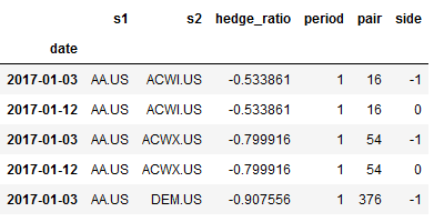
trades = pair_trade_data['side'].copy()
trades.loc[trades != 0] = 1
trades.loc[trades == 0] = -1
trades.sort_index().cumsum().plot(figsize=(14, 4))
sns.despine()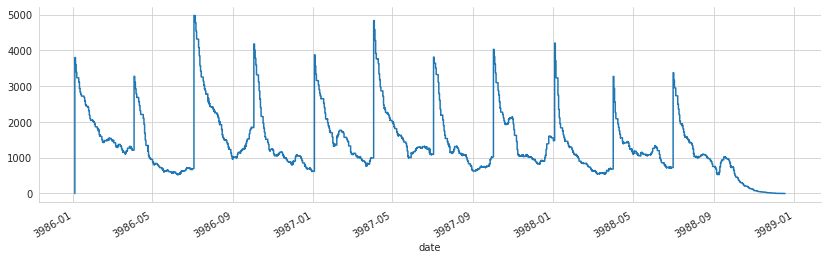
pair_trade_data.to_hdf('backtest.h5', 'pair_trades')この記事が気に入ったらサポートをしてみませんか?