
第11章:ランダムフォレスト - ロングショート戦略 第1節: 決定木と株価予想

はじめに
ここでは、決定木による株価予測モデルの構築とその評価について紹介します。
決定木には回帰と分類があって、回帰モデルの代表である最小二乗法による線形モデルと分類モデルの代表であるロジスティック回帰モデルと比較します。
ここでロジスティック回帰モデルが分類モデルであるにも関わらず、回帰と呼ばれている理由は、確率値を回帰して分類問題を解くからです。
基本的な内容から入るので結構長めの内容となっておりますが、初めての方でも参考になると思います(*'ω'*)
インポートと設定
import warnings
warnings.filterwarnings('ignore')
%matplotlib inline
import os, sys
from pathlib import Path
import numpy as np
from scipy.stats import spearmanr
import pandas as pd
import matplotlib.pyplot as plt
from matplotlib.ticker import FuncFormatter
from matplotlib import cm
import seaborn as sns
from sklearn.tree import DecisionTreeClassifier, DecisionTreeRegressor, export_graphviz, _tree
from sklearn.linear_model import LinearRegression, LogisticRegression
from sklearn.model_selection import train_test_split, GridSearchCV, learning_curve
from sklearn.metrics import roc_auc_score, roc_curve, mean_squared_error, make_scorer
import graphviz
import statsmodels.api as smsys.path.insert(1, os.path.join(sys.path[0], '..'))
from utils import MultipleTimeSeriesCVsns.set_style('white')results_path = Path('results', 'decision_trees')
if not results_path.exists():
results_path.mkdir(parents=True)モデルデータの読み込み
第4章のアルファーファクター研究で作成したデータセットの簡略版を使用します。これは、2010-2017年の期間にQuandlが提供する毎日の株価と、さまざまな設計機能で構成されています。詳細は、前の章に書いてあります。
この章の決定木モデルは、欠落変数またはカテゴリ変数を処理する機能を備えていないため、前者を削除した後で、後者にダミーエンコーディングを適用します。
with pd.HDFStore('data.h5') as store:
   data = store['us/equities/monthly']
data.info()
'''
<class 'pandas.core.frame.DataFrame'>
MultiIndex: 56756 entries, ('A', Timestamp('2010-12-31 00:00:00')) to ('ZION', Timestamp('2017-11-30 00:00:00'))
Data columns (total 27 columns):
#   Column         Non-Null Count  Dtype
---  ------         --------------  -----
0   atr            56756 non-null  float64
1   bb_down        56756 non-null  float64
2   bb_high        56756 non-null  float64
3   bb_low         56756 non-null  float64
4   bb_mid         56756 non-null  float64
5   bb_up          56756 non-null  float64
6   macd           56756 non-null  float64
7   natr           56756 non-null  float64
8   rsi            56756 non-null  float64
9   sector         56756 non-null  object
10  return_1m      56756 non-null  float64
11  return_3m      56756 non-null  float64
12  return_6m      56756 non-null  float64
13  return_12m     56756 non-null  float64
14  beta           56756 non-null  float64
15  SMB            56756 non-null  float64
16  HML            56756 non-null  float64
17  RMW            56756 non-null  float64
18  CMA            56756 non-null  float64
19  momentum_3     56756 non-null  float64
20  momentum_6     56756 non-null  float64
21  momentum_3_6   56756 non-null  float64
22  momentum_12    56756 non-null  float64
23  momentum_3_12  56756 non-null  float64
24  year           56756 non-null  int64
25  month          56756 non-null  int64
26  target         56756 non-null  float64
dtypes: float64(24), int64(2), object(1)
memory usage: 12.0+ MB
'''
単純回帰木予測
ここでは一か月後予測をします。
X2 = data.loc[:, ['target', 'return_1m']]
X2.columns = ['y', 't-1']
X2['t-2'] = data.groupby(level='ticker').return_1m.shift()
X2 = X2.dropna()
X2.info()
'''
<class 'pandas.core.frame.DataFrame'>
MultiIndex: 56186 entries, ('A', Timestamp('2011-01-31 00:00:00')) to ('ZION', Timestamp('2017-11-30 00:00:00'))
Data columns (total 3 columns):
#   Column  Non-Null Count  Dtype
---  ------  --------------  -----
0   y       56186 non-null  float64
1   t-1     56186 non-null  float64
2   t-2     56186 non-null  float64
dtypes: float64(3)
memory usage: 1.5+ MB
'''
y2 = X2.y
X2 = X2.drop('y', axis=1)データを見てみる
sns.distplot(y2)
sns.despine();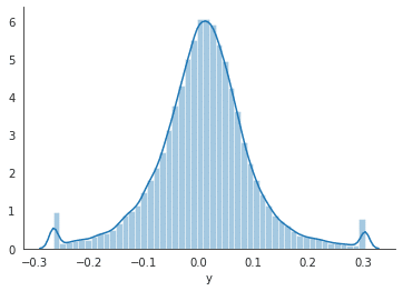
ツリーの設定
reg_tree_t2 = DecisionTreeRegressor(criterion='mse',
                                   splitter='best',
                                   max_depth=6,
                                   min_samples_split=2,
                                   min_samples_leaf=50,
                                   min_weight_fraction_leaf=0.0,
                                   max_features=None,
                                   random_state=42,
                                   max_leaf_nodes=None,
                                   min_impurity_decrease=0.0,
                                   min_impurity_split=None,
                                   presort=False)
訓練する
reg_tree_t2.fit(X=X2, y=y2)ツリーを視覚化する
out_file = results_path / 'reg_tree_t2.dot'
dot_data = export_graphviz(reg_tree_t2,
                         out_file=out_file.as_posix(),
                         feature_names=X2.columns,
                         max_depth=2,
                         filled=True,
                         rounded=True,
                         special_characters=True)
if out_file is not None:
   dot_data = Path(out_file).read_text()

graphviz.Source(dot_data)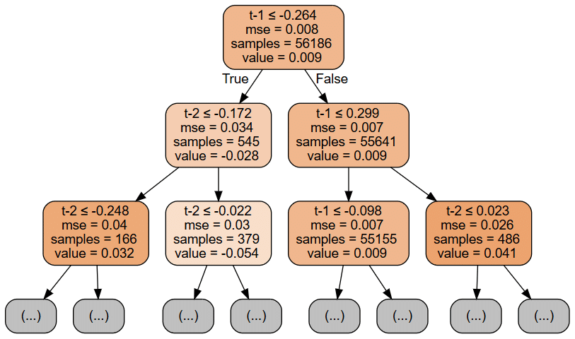
線形回帰と比較する
以下のOLSの概要と上の決定木の最初の2つの層を視覚化すると、モデル間の顕著な違いがわかります。 OLSモデルは、切片の3つのパラメーターと、線形仮定に沿った2つの特徴を提供します。
対照的に、上記の回帰ツリーグラフは、最初の2つのレベルの各ノードについて、データを分割するために使用される機能としきい値(機能は繰り返し使用できることに注意してください)と平均二乗誤差(MSE)の現在の値を表示します)、サンプル数、およびこれらのトレーニングサンプルに基づく予測値。
また、ツリーチャートは、2つの分割のみの後に数が31,000から65,000サンプルの間で変化するため、ノード全体のサンプルの不均一な分布を強調表示します。
statsmodels OLS
ols_model = sm.OLS(endog=y2, exog=sm.add_constant(X2))result = ols_model.fit()
print(result.summary())
'''
OLS Regression Results
==============================================================================
Dep. Variable: y R-squared: 0.001
Model: OLS Adj. R-squared: 0.001
Method: Least Squares F-statistic: 39.02
Date: Thu, 20 Aug 2020 Prob (F-statistic): 1.17e-17
Time: 13:28:45 Log-Likelihood: 56967.
No. Observations: 56186 AIC: -1.139e+05
Df Residuals: 56183 BIC: -1.139e+05
Df Model: 2
Covariance Type: nonrobust
==============================================================================
coef std err t P>|t| [0.025 0.975]
------------------------------------------------------------------------------
const 0.0088 0.000 23.412 0.000 0.008 0.009
t-1 0.0327 0.004 7.761 0.000 0.024 0.041
t-2 -0.0187 0.004 -4.437 0.000 -0.027 -0.010
==============================================================================
Omnibus: 2103.126 Durbin-Watson: 1.999
Prob(Omnibus): 0.000 Jarque-Bera (JB): 6483.607
Skew: 0.018 Prob(JB): 0.00
Kurtosis: 4.664 Cond. No. 11.5
==============================================================================
'''sklearn 線形回帰
lin_reg = LinearRegression()lin_reg.fit(X=X2,y=y2)lin_reg.intercept_
'''
0.008755441196301639
'''lin_reg.coef_
'''
array([ 0.03269516, -0.01868576])
'''識別境界 線形回帰 vs 回帰木
入力変数と出力の間の関係の関数形式に関するさまざまな仮定をさらに説明するために、現在のリターン予測を特徴空間の関数として、つまり遅延リターンの値の範囲の関数として視覚化できます。 次の図は、線形回帰と回帰木の1と2期間前のリターンの関数としての現在の期間のリターンを示しています。
右側の線形回帰モデルの結果は、時間差と現在のリターン間の関係の線形性を強調していますが、左側の回帰ツリーチャートは、特徴空間の再帰的分割でエンコードされた非線形関係を示しています。
t1, t2 = np.meshgrid(np.linspace(X2['t-1'].quantile(.01), X2['t-1'].quantile(.99), 100),
                    np.linspace(X2['t-2'].quantile(.01), X2['t-2'].quantile(.99), 100))
X_data = np.c_[t1.ravel(), t2.ravel()]
fig, axes = plt.subplots(ncols=2, figsize=(12,5))
# Linear Regression
ret1 = lin_reg.predict(X_data).reshape(t1.shape)
surface1 = axes[0].contourf(t1, t2, ret1, cmap='Blues')
plt.colorbar(mappable=surface1, ax=axes[0])
# Regression Tree
ret2 = reg_tree_t2.predict(X_data).reshape(t1.shape)
surface2 = axes[1].contourf(t1, t2, ret2, cmap='Blues')
plt.colorbar(mappable=surface2, ax=axes[1])
# Format plots
titles = ['Linear Regression', 'Regression Tree']
for i, ax in enumerate(axes):
ax.set_xlabel('t-1')
ax.set_ylabel('t-2')
ax.set_title(titles[i])
fig.suptitle('Decision Surfaces', fontsize=14)
sns.despine()
fig.tight_layout()
fig.subplots_adjust(top=.9);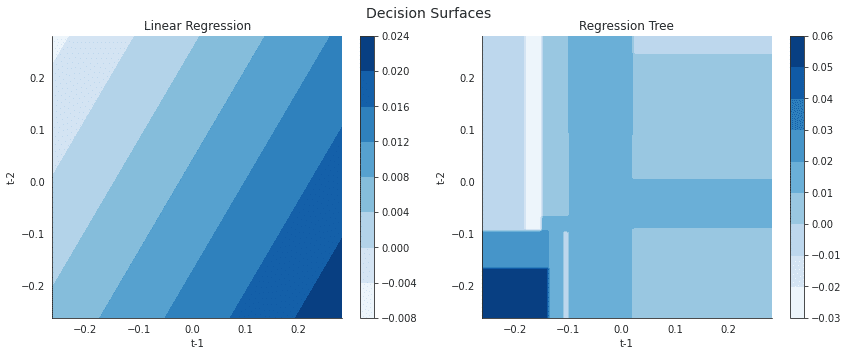
単純分類木
分類木は回帰バージョンと似ていますが、異なる点として、結果のカテゴリカルな性質(例. 0か1)の予測と損失関数の評価で異なるアプローチをとります。
回帰木は、関連する訓練サンプルの平均結果を使用して葉ノードに割り当てられた観測の応答を予測しますが、分類木は代わりにモード、つまり関連する領域の訓練サンプルの中で最も一般的なクラスを使用します。分類ツリーは、相対クラス頻度に基づいて確率的予測を生成することもできます。
損失関数
分類木を成長させるときは、再帰的なバイナリ分割も使用しますが、平均二乗誤差の低減を使用して決定ルールの品質を評価する代わりに、誤分類率(misclassification rate)(最も大きいクラスに属していないサンプルの割合)を使用できます。
ただし、ジニ係数またはクロスエントロピーという代替指標は、分類エラー率よりもノードの純度に敏感であるため、推奨されます。ノードの純粋性は、ノード内の単一のクラスの優勢の程度を指します。単一のクラスに属する結果を持つサンプルのみを含むノードは純粋であり、特徴空間のこの特定の領域の分類が成功したことを意味します。
ここでは有名な三つの評価関数を定義します。(二値分類)
def entropy(f):
   return (-f*np.log2(f) - (1-f)*np.log2(1-f))/2
def gini(f):
return 2*f*(1-f)def misclassification_rate(f):
return np.where(f<=.5, f, 1-f)x = np.linspace(0, 1, 10000)
(pd.DataFrame({'Gini': gini(x),
'Entropy': entropy(x),
'Misclassification Rate': misclassification_rate(x)}, index=x)
.plot(title='Classification Loss Functions', lw=2, style=['-', '--', ':']))
sns.despine()
plt.tight_layout();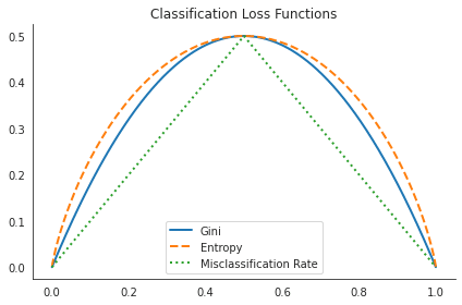
分類木の設定
clf_tree_t2 = DecisionTreeClassifier(criterion='gini',
                                    splitter='best',
                                    max_depth=5,
                                    min_samples_split=1000,
                                    min_samples_leaf=1,
                                    min_weight_fraction_leaf=0.0,
                                    max_features=None,
                                    random_state=42,
                                    max_leaf_nodes=None,
                                    min_impurity_decrease=0.0,
                                    min_impurity_split=None,
                                    class_weight=None,
                                    presort=False)
y_binary = (y2>0).astype(int)
y_binary.value_counts()
'''
1 31568
0 24618
Name: y, dtype: int64
'''clf_tree_t2.fit(X=X2, y=y_binary)ツリーの視覚化
out_file = results_path / 'clf_tree_t2.dot'
dot_data = export_graphviz(clf_tree_t2,
                          out_file=out_file.as_posix(),
                          feature_names=X2.columns,
                          class_names=['Down', 'Up'],
                          max_depth=2,
                          filled=True,
                          rounded=True,
                          special_characters=True)
if out_file is not None:
   dot_data = Path(out_file).read_text()

graphviz.Source(dot_data)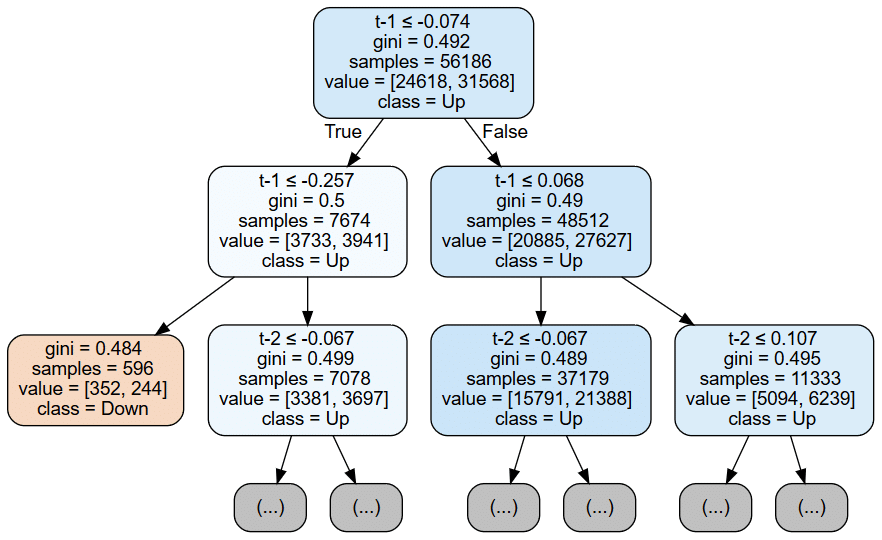
ロジスティック回帰と比較
statsmodels
log_reg_sm = sm.Logit(endog=y_binary, exog=sm.add_constant(X2))log_result = log_reg_sm.fit()
'''
Optimization terminated successfully.
Current function value: 0.685280
Iterations 4
'''print(log_result.summary())
'''
Logit Regression Results
==============================================================================
Dep. Variable: y No. Observations: 56186
Model: Logit Df Residuals: 56183
Method: MLE Df Model: 2
Date: Thu, 20 Aug 2020 Pseudo R-squ.: 0.0002871
Time: 13:29:48 Log-Likelihood: -38503.
converged: True LL-Null: -38514.
Covariance Type: nonrobust LLR p-value: 1.578e-05
==============================================================================
coef std err z P>|z| [0.025 0.975]
------------------------------------------------------------------------------
const 0.2447 0.009 28.513 0.000 0.228 0.262
t-1 0.4548 0.097 4.698 0.000 0.265 0.644
t-2 0.0018 0.097 0.019 0.985 -0.188 0.191
==============================================================================
'''sklearn
log_reg_sk = LogisticRegression()log_reg_sk.fit(X=X2, y=y_binary)log_reg_sk.coef_
'''
array([[0.45052983, 0.0019411 ]])
'''識別境界: 分類木 vs. ロジスティック回帰
fig, axes = plt.subplots(ncols=2, figsize=(12,5))

# Linear Regression
ret1 = log_reg_sk.predict_proba(X_data)[:, 1].reshape(t1.shape)
surface1 = axes[0].contourf(t1, t2, ret1, cmap='Blues')
plt.colorbar(mappable=surface1, ax=axes[0])

# Regression Tree
ret2 = clf_tree_t2.predict_proba(X_data)[:, 1].reshape(t1.shape)
surface2 = axes[1].contourf(t1, t2, ret2, cmap='Blues')
plt.colorbar(mappable=surface2, ax=axes[1])

# Format plots
titles = ['Logistic Regression', 'Classification Tree']
for i, ax in enumerate(axes):
   ax.set_xlabel('t-1')
   ax.set_ylabel('t-2')
   ax.set_title(titles[i])

fig.suptitle('Decision Surfaces', fontsize=20)
sns.despine()
fig.tight_layout()
fig.subplots_adjust(top=.9);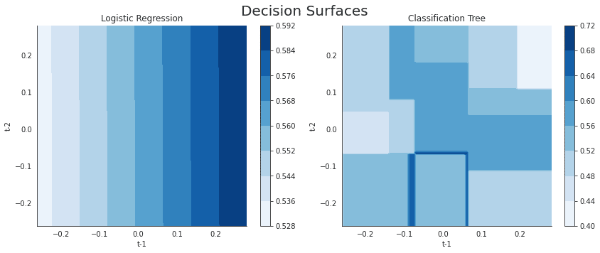
全ての特徴量で回帰木
80%訓練、20%テスト期間とします。
X = pd.get_dummies(data.drop('target', axis=1))
y = data.target
X_train, X_test, y_train, y_test = train_test_split(X, y, test_size=0.2, random_state=42)ツリーの設定
regression_tree = DecisionTreeRegressor(criterion='mse',
                                       splitter='best',
                                       max_depth=5,
                                       min_samples_split=2,
                                       min_samples_leaf=1,
                                       min_weight_fraction_leaf=0.0,
                                       max_features=None,
                                       random_state=42,
                                       max_leaf_nodes=None,
                                       min_impurity_decrease=0.0,
                                       min_impurity_split=None,
                                       presort=False)
モデルの訓練
regression_tree.fit(X=X_train, y=y_train)ツリーの視覚化
out_file = results_path / 'reg_tree.dot'
dot_data = export_graphviz(regression_tree,
                          out_file=out_file.as_posix(),
                          feature_names=X_train.columns,
                          max_depth=3,
                          filled=True,
                          rounded=True,
                          special_characters=True)
if out_file is not None:
   dot_data = Path(out_file).read_text()

graphviz.Source(dot_data)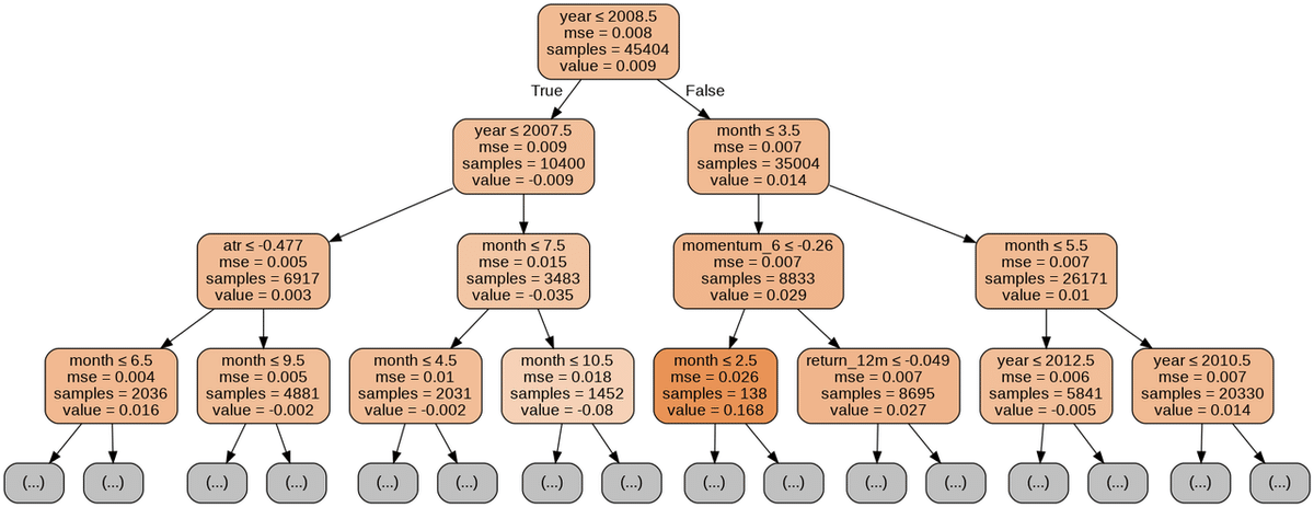
テストセットの評価
y_pred = regression_tree.predict(X_test)np.sqrt(mean_squared_error(y_pred=y_pred, y_true=y_test))
'''
0.08086872759273504
'''r, p = spearmanr(y_pred, y_test)
print(f'{r*100:.2f} (p-value={p:.2%})')
'''
27.73 (p-value=0.00%)
'''全ての特徴量で分類木
y_binary = (y>0).astype(int)
y_binary.value_counts()
X_train, X_test, y_train, y_test = train_test_split(X, y_binary, test_size=0.2, random_state=42)clf = DecisionTreeClassifier(criterion='gini',
max_depth=5,
random_state=42)clf.fit(X=X_train, y=y_train)out_file = results_path / 'clf_tree.dot'
dot_data = export_graphviz(clf,
out_file=out_file.as_posix(),
feature_names=X.columns,
class_names=['Down', 'Up'],
max_depth=3,
filled=True,
rounded=True,
special_characters=True)
if out_file is not None:
dot_data = Path(out_file).read_text()
graphviz.Source(dot_data)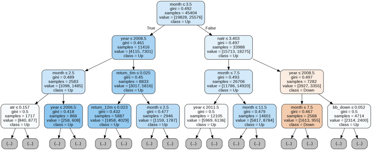
テストセット評価
y_score = clf.predict_proba(X=X_test)[:, 1]roc_auc_score(y_score=y_score, y_true=y_test)
'''
0.6314068026403399
'''識別パスの出力
from sklearn.tree._tree import Treedef tree_to_code(tree, feature_names):
if isinstance(tree, DecisionTreeClassifier):
model = 'clf'
elif isinstance(tree, DecisionTreeRegressor):
model = 'reg'
else:
raise ValueError('Need Regression or Classification Tree')
tree_ = tree.tree_
feature_name = [
feature_names[i] if i != _tree.TREE_UNDEFINED else "undefined!"
for i in tree_.feature
]
print("def tree({}):".format(", ".join(feature_names)))
def recurse(node, depth):
indent = " " * depth
if tree_.feature[node] != _tree.TREE_UNDEFINED:
name = feature_name[node]
threshold = tree_.threshold[node]
print(indent, f'if {name} <= {threshold:.2%}')
recurse(tree_.children_left[node], depth + 1)
print(indent, f'else: # if {name} > {threshold:.2%}')
recurse(tree_.children_right[node], depth + 1)
else:
pred = tree_.value[node][0]
val = pred[1]/sum(pred) if model == 'clf' else pred[0]
print(indent, f'return {val:.2%}')
recurse(0, 1)tree_to_code(clf_tree_t2, X2.columns)
'''
def tree(t-1, t-2):
if t-1 <= -7.44%
if t-1 <= -25.72%
return 40.94%
else: # if t-1 > -25.72%
if t-2 <= -6.72%
if t-1 <= -8.81%
if t-1 <= -8.88%
return 55.26%
else: # if t-1 > -8.88%
return 23.08%
else: # if t-1 > -8.81%
return 64.47%
else: # if t-2 > -6.72%
if t-1 <= -13.61%
if t-2 <= 4.83%
return 44.72%
else: # if t-2 > 4.83%
return 50.09%
else: # if t-1 > -13.61%
if t-2 <= 8.26%
return 51.19%
else: # if t-2 > 8.26%
return 56.97%
else: # if t-1 > -7.44%
if t-1 <= 6.76%
if t-2 <= -6.66%
if t-1 <= 6.15%
if t-1 <= -7.16%
return 72.22%
else: # if t-1 > -7.16%
return 54.31%
else: # if t-1 > 6.15%
return 66.46%
else: # if t-2 > -6.66%
if t-2 <= -6.11%
return 68.22%
else: # if t-2 > -6.11%
if t-2 <= 17.86%
return 57.84%
else: # if t-2 > 17.86%
return 53.04%
else: # if t-1 > 6.76%
if t-2 <= 10.66%
if t-2 <= -10.81%
if t-1 <= 28.33%
return 50.88%
else: # if t-1 > 28.33%
return 62.29%
else: # if t-2 > -10.81%
if t-2 <= 3.57%
return 57.25%
else: # if t-2 > 3.57%
return 53.67%
else: # if t-2 > 10.66%
if t-1 <= 18.83%
return 51.39%
else: # if t-1 > 18.83%
return 43.17%
'''過学習、正則化とパラメーターチューニング
ここでパラメーターチューニングするために、決定木にどんなパラメーターがあるのかについて見ていきましょう。
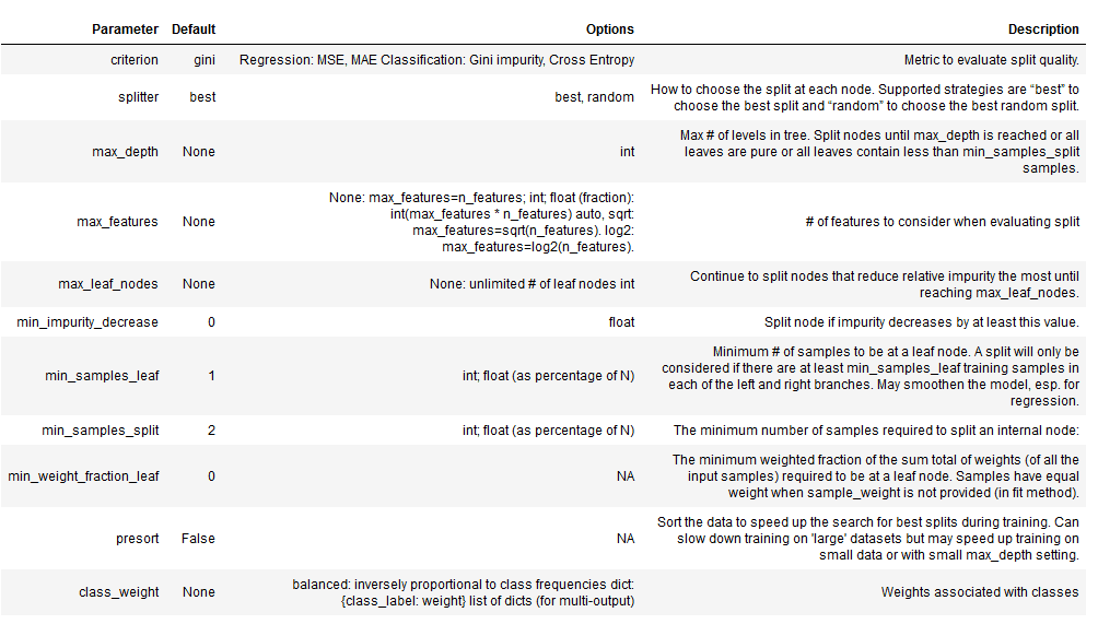
max_depthパラメーターは、連続する分割の数にハード制限を課し、ツリーの成長を制限する最も簡単な方法を表します。
min_samples_splitおよびmin_samples_leafパラメータは、ツリーの成長を制限するための代替のデータ駆動型の方法です。これらのパラメーターは、連続する分割の数に厳しい制限を課すのではなく、データをさらに分割するために必要なサンプルの最小数を制御します。後者は葉ごとに特定の数のサンプルを保証しますが、前者は分割によって非常に不均一な分布が生じる場合、非常に小さな葉を作成できます。パラメーター値が小さいとオーバーフィッティングが容易になりますが、数値が大きいとツリーがデータの信号を学習できなくなる可能性があります。
多くの場合、デフォルト値は非常に低いため、交差検証を使用して潜在的な値の範囲を調査する必要があります。絶対値ではなく、フロート(float)を使用してパーセンテージを示すこともできます。
交差検定パラメーター
n_splits = 10
train_period_length = 60
test_period_length = 6
lookahead = 1

cv = MultipleTimeSeriesCV(n_splits=n_splits,
                         train_period_length=train_period_length,
                         test_period_length=test_period_length,
                         lookahead=lookahead)
max_depths = range(1, 16)GridSearchCVを利用して最適な木を探す
パラメーターグリッドの定義
param_grid = {'max_depth': [2, 3, 4, 5, 6, 7, 8, 10, 12, 15],
             'min_samples_leaf': [5, 25, 50, 100],
             'max_features': ['sqrt', 'auto']}
分類木
clf = DecisionTreeClassifier(random_state=42)次に、GridSearchCVオブジェクトをインスタンス化して、推定子オブジェクトとパラメーターグリッドを提供するとともに、スコアリングメソッドと交差検証の選択肢を初期化メソッドに提供します。カスタムOneStepTimeSeriesSplitクラスのオブジェクトを使用し、cvパラメーターに10倍を使用するように初期化し、スコアリングをroc_aucメトリックに設定します。 n_jobsパラメーターを使用して検索を並列化し、refit = Trueを設定することにより、最適なハイパーパラメーターを使用するトレーニング済みモデルを自動的に取得できます。
gridsearch_clf = GridSearchCV(estimator=clf,
                         param_grid=param_grid,
                         scoring='roc_auc',
                         n_jobs=-1,
                         cv=cv,
                         refit=True,
                         return_train_score=True)
gridsearch_clf.fit(X=X, y=y_binary)
'''
GridSearchCV(cv=<utils.MultipleTimeSeriesCV object at 0x7f17dc1cb950>,
estimator=DecisionTreeClassifier(random_state=42), n_jobs=-1,
param_grid={'max_depth': [2, 3, 4, 5, 6, 7, 8, 10, 12, 15],
'max_features': ['sqrt', 'auto'],
'min_samples_leaf': [5, 25, 50, 100]},
return_train_score=True, scoring='roc_auc')
'''訓練の過程では、GridSearchCVオブジェクトのいくつかの新しい属性を生成します。最も重要なのは、最適な設定と最高の相互検証スコアに関する情報です(先読みバイアスを回避する適切な設定を使用しています)。
max_depthを10に、min_samples_leafを5に設定し、分割を決定するときに特徴量の総数の平方根に対応する数のみをランダムに選択すると、AUCが0.5263の最良の結果が得られます。
gridsearch_clf.best_params_
'''
{'max_depth': 12, 'max_features': 'sqrt', 'min_samples_leaf': 5}
'''
gridsearch_clf.best_score_
'''
0.5263050084776537
'''カスタムICスコアの定義
def rank_correl(y, y_pred):
   return spearmanr(y, y_pred)[0]
ic = make_scorer(rank_correl)
回帰木
reg_tree = DecisionTreeRegressor(random_state=42)gridsearch_reg = GridSearchCV(estimator=reg_tree,
param_grid=param_grid,
scoring=ic,
n_jobs=-1,
cv=cv,
refit=True,
return_train_score=True)gridsearch_reg.fit(X=X, y=y)
'''
GridSearchCV(cv=<utils.MultipleTimeSeriesCV object at 0x7f17dc1cb950>,
estimator=DecisionTreeRegressor(random_state=42), n_jobs=-1,
param_grid={'max_depth': [2, 3, 4, 5, 6, 7, 8, 10, 12, 15],
'max_features': ['sqrt', 'auto'],
'min_samples_leaf': [5, 25, 50, 100]},
return_train_score=True, scoring=make_scorer(rank_correl))
'''gridsearch_reg.best_params_
'''
{'max_depth': 6, 'max_features': 'sqrt', 'min_samples_leaf': 50}
'''gridsearch_reg.best_score_
'''
0.08415538441512119
'''pd.DataFrame({'Regression': pd.Series(gridsearch_reg.best_params_),
'Classification': pd.Series(gridsearch_clf.best_params_)})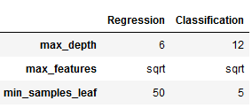
分類木交差検定
def get_leaves_count(tree):
   t = tree.tree_
   n = t.node_count
   leaves = len([i for i in range(t.node_count) if t.children_left[i]== -1])
   return leaves
train_scores, val_scores, leaves = {}, {}, {}
for max_depth in max_depths:
print(max_depth, end=' ', flush=True)
clf = DecisionTreeClassifier(criterion='gini',
max_depth=max_depth,
min_samples_leaf=5,
max_features='sqrt',
random_state=42)
train_scores[max_depth], val_scores[max_depth], leaves[max_depth] = [], [], []
for train_idx, test_idx in cv.split(X):
X_train, y_train, = X.iloc[train_idx], y_binary.iloc[train_idx]
X_test, y_test = X.iloc[test_idx], y_binary.iloc[test_idx]
clf.fit(X=X_train, y=y_train)
train_pred = clf.predict_proba(X=X_train)[:, 1]
train_score = roc_auc_score(y_score=train_pred, y_true=y_train)
train_scores[max_depth].append(train_score)
test_pred = clf.predict_proba(X=X_test)[:, 1]
val_score = roc_auc_score(y_score=test_pred, y_true=y_test)
val_scores[max_depth].append(val_score)
leaves[max_depth].append(get_leaves_count(clf))
clf_train_scores = pd.DataFrame(train_scores)
clf_valid_scores = pd.DataFrame(val_scores)
clf_leaves = pd.DataFrame(leaves)
'''
1 2 3 4 5 6 7 8 9 10 11 12 13 14 15
'''clf_cv_data = pd.concat([pd.melt(clf_train_scores,
var_name='Max. Depth',
value_name='ROC AUC').assign(Data='Train'),
pd.melt(clf_valid_scores,
var_name='Max. Depth',
value_name='ROC AUC').assign(Data='Valid')])回帰木交差検定
train_scores, val_scores, leaves = {}, {}, {}
for max_depth in max_depths:
   print(max_depth, end=' ', flush=True)
   reg_tree = DecisionTreeRegressor(max_depth=max_depth,
                                    min_samples_leaf=50,
                                    max_features= 'sqrt',
                                    random_state=42)
   train_scores[max_depth], val_scores[max_depth], leaves[max_depth] = [], [], []
   for train_idx, test_idx in cv.split(X):
       X_train, y_train,  = X.iloc[train_idx], y.iloc[train_idx]
       X_test, y_test = X.iloc[test_idx], y.iloc[test_idx]
       reg_tree.fit(X=X_train, y=y_train)

       train_pred = reg_tree.predict(X=X_train)
       train_score = spearmanr(train_pred, y_train)[0]
       train_scores[max_depth].append(train_score)

       test_pred = reg_tree.predict(X=X_test)
       val_score = spearmanr(test_pred, y_test)[0]
       val_scores[max_depth].append(val_score)
       leaves[max_depth].append(get_leaves_count(reg_tree))

reg_train_scores = pd.DataFrame(train_scores)
reg_valid_scores = pd.DataFrame(val_scores)
reg_leaves = pd.DataFrame(leaves)
'''
1 2 3 4 5 6 7 8 9 10 11 12 13 14 15
'''
reg_cv_data = (pd.melt(reg_train_scores, var_name='Max. Depth',
value_name='IC').assign(Data='Train').append(
pd.melt(reg_valid_scores,
var_name='Max. Depth',
value_name='IC').assign(Data='Valid')))
交差検定 : 回帰木 vs 分類木の比較
fig, axes = plt.subplots(ncols=2, figsize=(14, 5))

sns.lineplot(data=reg_cv_data,
            x='Max. Depth', y='IC',
            hue='Data', ci=95,
            ax=axes[0], lw=2)

axes[0].set_title('Regression Tree')
axes[0].axvline(x=reg_valid_scores.mean().idxmax(), ls='--', c='k', lw=1)
axes[0].axhline(y=0, ls='--', c='k', lw=1)

sns.lineplot(data=clf_cv_data,
            x='Max. Depth', y='ROC AUC',
            hue='Data', ci=95,
            ax=axes[1], lw=2)

axes[1].set_title('Classification Tree')
axes[1].axvline(x=clf_valid_scores.mean().idxmax(), ls='--', c='k', lw=1)
axes[1].axhline(y=.5, ls='--', c='k', lw=1)
for ax in axes:
   ax.set_xlim(min(param_grid['max_depth']),
               max(param_grid['max_depth']))

fig.suptitle(f'Train-Validation Scores', fontsize=14)
sns.despine()
fig.tight_layout()
fig.subplots_adjust(top=.91)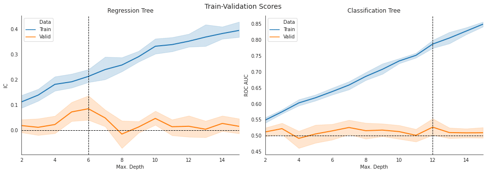
最適モデルの学習曲線
sizes = np.arange(.1, 1.01, .1)train_sizes, train_scores, valid_scores = learning_curve(gridsearch_clf.best_estimator_,
X,
y_binary,
train_sizes=sizes,
cv=cv,
scoring='roc_auc',
n_jobs=-1,
shuffle=True,
random_state=42)clf_lc_data = pd.concat([
pd.melt(pd.DataFrame(train_scores.T, columns=train_sizes),
var_name='Train Size',
value_name='ROC AUC').assign(Data='Train'),
pd.melt(pd.DataFrame(valid_scores.T, columns=train_sizes),
var_name='Train Size',
value_name='ROC AUC').assign(Data='Valid')])
clf_lc_data.info()
'''
<class 'pandas.core.frame.DataFrame'>
Int64Index: 200 entries, 0 to 99
Data columns (total 3 columns):
# Column Non-Null Count Dtype
--- ------ -------------- -----
0 Train Size 200 non-null int64
1 ROC AUC 200 non-null float64
2 Data 200 non-null object
dtypes: float64(1), int64(1), object(1)
memory usage: 6.2+ KB
'''回帰木
train_sizes, train_scores, valid_scores = learning_curve(gridsearch_reg.best_estimator_,
                                                        X, y,
                                                        train_sizes=sizes,
                                                        cv=cv,
                                                        scoring=ic,
                                                        n_jobs=-1,
                                                        shuffle=True,
                                                        random_state=42)
reg_lc_data = pd.concat([
pd.melt(pd.DataFrame(train_scores.T,
columns=train_sizes),
var_name='Train Size',
value_name='IC').assign(Data='Train'),
pd.melt(pd.DataFrame(valid_scores.T,
columns=train_sizes),
var_name='Train Size',
value_name='IC').assign(Data='Valid')])
reg_lc_data.info()
'''
<class 'pandas.core.frame.DataFrame'>
Int64Index: 200 entries, 0 to 99
Data columns (total 3 columns):
# Column Non-Null Count Dtype
--- ------ -------------- -----
0 Train Size 200 non-null int64
1 IC 200 non-null float64
2 Data 200 non-null object
dtypes: float64(1), int64(1), object(1)
memory usage: 6.2+ KB
'''学習曲線比較
fig, axes = plt.subplots(ncols=2, figsize=(14, 5))
xmin, xmax = reg_lc_data['Train Size'].min(), reg_lc_data['Train Size'].max()

sns.lineplot(data=reg_lc_data,
            x='Train Size', y='IC',
            hue='Data', ci=95,  ax=axes[0], lw=2)
axes[0].set_title('Best Regression Tree')
axes[0].set_ylabel('IC')

axes[0].xaxis.set_major_formatter(
   FuncFormatter(lambda x, _: '{:,.0f}'.format(x)))

sns.lineplot(data=clf_lc_data,
            x='Train Size',
            y='ROC AUC',
            hue='Data',
            ci=95,
            ax=axes[1],
            lw=2)
axes[1].set_title('Best Classification Tree')
axes[1].set_ylabel('ROC AUC')
axes[1].xaxis.set_major_formatter(
   FuncFormatter(lambda x, _: '{:,.0f}'.format(x)))

for i in [0, 1]:
   axes[i].tick_params(axis='both', which='major', labelsize=10)
   axes[i].tick_params(axis='both', which='minor', labelsize=8)
   axes[i].set_xlim(xmin, xmax)

fig.suptitle('Learning Curves', fontsize=14)
sns.despine()
fig.tight_layout()
fig.subplots_adjust(top=.9)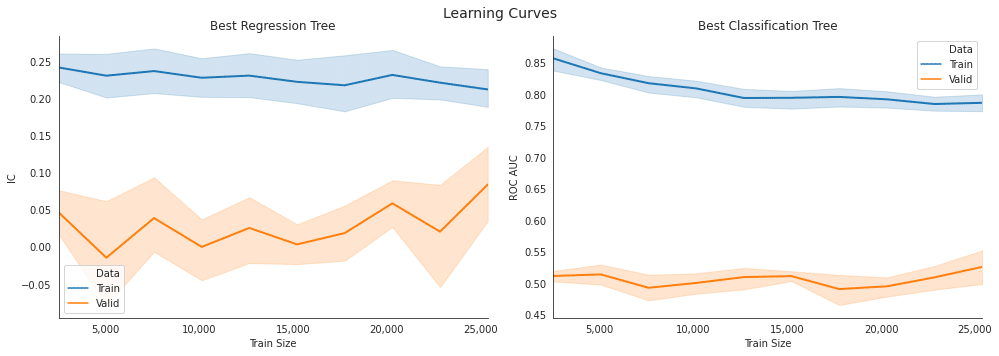
特徴量の重要度
top_n = 15
labels = X.columns.str.replace('_', ' ').str.upper()
fi_clf = (pd.Series(gridsearch_clf.best_estimator_.feature_importances_,
                   index=labels).sort_values(ascending=False).iloc[:top_n])
fi_reg = (pd.Series(gridsearch_reg.best_estimator_.feature_importances_,
                   index=labels).sort_values(ascending=False).iloc[:top_n])
fig, axes= plt.subplots(ncols=2, figsize=(12,4), sharex=True)
color = cm.Blues(np.linspace(.4,.9, top_n))
fi_clf.sort_values().plot.barh(ax=axes[1], title='Classification Tree', color=color)
fi_reg.sort_values().plot.barh(ax=axes[0], title='Regression Tree', color=color)
axes[0].set_xlabel('Feature Importance')
axes[1].set_xlabel('Feature Importance')
fig.suptitle(f'Top {top_n} Features', fontsize=14)
sns.despine()
fig.tight_layout()
fig.subplots_adjust(top=.9);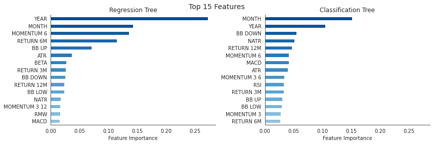
この記事が気に入ったらサポートをしてみませんか?