
Fat tailを仕留めたい!

The history of the distribution of wealth has always been deeply political, and it cannot be reduced to purely economic mechanisms.
金融市場において、株価や収益率の分布を単なる正規分布だけで説明するのは不十分である。これは、実際の市場データをみると、正規分布が想定するよりはるかに極端な変動が頻繁に起こるfat tailと呼ばれる特徴によるものである。
正規分布では3σを超えるような値は理論上ごく稀であるが、実際の株価変動ではこうした極端な変動が意外に頻繁に観測される。その結果、リスク評価の際に「株価や収益率は正規分布に従う」と単純に仮定してしまうと、このfat tailに含まれる極端な損失リスクを過小評価してしまう恐れがある。(因みにBlack Scholes方程式は正規分布を仮定している。)
そこで、fat tailを適切に捉えられるような分布を用いることで、より現実的なリスク管理に応用できる可能性がある。
余談:こうした極端なリスクを論じる際によく話題になるのが、Nassim Nicholas Talebによって提唱されたBlack Swanの概念である。Black Swanはそれまで存在しないと信じられていた、極端に稀かつ予測不可能で、起こると甚大な影響を及ぼす出来事を指す。しかし、スイスの物理学者であるDidier Sornetteは、これらの極端な出来事の一部はまったく予測不能ではないと主張している。Sornetteは、表面的にはBlack Swanに見えるが、詳細な分析により予測が可能になるタイプの出来事をDragon Kingと呼んでいる。
では、 実際のデータにみられるfat tailをうまく捉えるには、どのような分布を用いればよいのか。ここでは、代表的な分布(scipy statsにある) としてGaussian、Student’s t、Laplace、GED、NIG、GH、Levy安定分布の7つを取り上げて、どの程度fat tailを捉えられるかを比較してみたい。
各分布
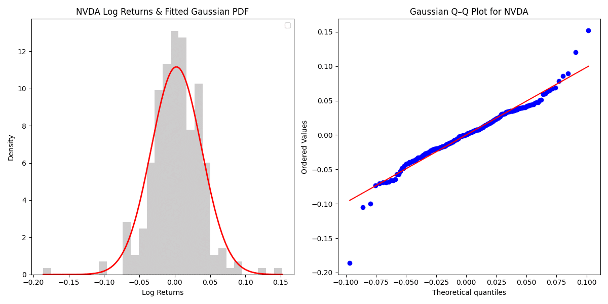
Gaussian
fat tailを十分に表現できない。

Student's t
$$自由度\nuを小さくすれば裾が厚くなりfattailを捉えることができる。
\nuを無限大にすれば正規分布に近似可能である。$$

Laplace

GED: Generalized Normal
$$\beta=2で正規分布に一致し、\beta<2で裾が厚くなる。$$

NIG: Normal Inverse Gaussian

GH: Generalized Hyperbolic

Levy 安定
Levy分布は確率密度関数を持たず、その代わりに特性関数で定義される。
fat tailを捉える最適な分布の一つとして知られている。

$$\alphaは安定性パラメータであり、2の時正規分布に一致する。
\betaは歪度パラメータで[-1,1]の範囲で値を取る。基本的に、\alpha <2の時は裾が暑くなる。解析解が存在しないため数値計算による近似が必要である。$$
この他にGHの下位互換としてVG(Variance Gamma)という分布があるが、Scipy.statsのライブラリーには未だ含まれていないため今回は取り扱わない。(Rにはある。)
株価収益率をfittingする
ここでは、例として過去一年間のNVDAの対数収益率を上記の分布を用いてfittingする。以下に、fittingした結果と各々のqq-plotを示した。


統計量による比較
AIC/BICとKS統計量で各々の分布の適合度合いを比較した。

表より以下のことが明らかになった。
AIC/BICとKS統計量の観点からはStudent’s tが最も良い適合度を示している。
LevyとGEDも比較的適合している。
結論として、NVDAの場合はStudent's tが優れている。