
【ファイル付き】コピペで使えるExcelマクロ!ガントチャート自動作成・更新マクロ

ガントチャートは、プロジェクト管理やタスク管理でよく用いられるツールで、タスクの開始日・終了日や進捗を視覚的に把握するのにとても便利です。
しかし「Excelでガントチャートを作ろう」と思っても、日付をひとつずつ設定したりセルを色分けしたりと手間がかかりがちですよね。
そこで今回は、VBA(Excelのマクロ機能)を使ってボタンひとつでガントチャートを自動生成するマクロをご紹介します。
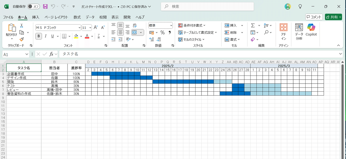
実際にExcelマクロで作成されるガントチャートのイメージ図です。
このシートは一切人の手で操作していません。
こんな図が、マクロで一発で作れるようになります!
どうがはこちらから
Excelマクロの基本的な使い方は、下の記事を参考にしてください
1. マクロの概要
今回紹介するマクロは、以下のような流れでガントチャートを生成します。
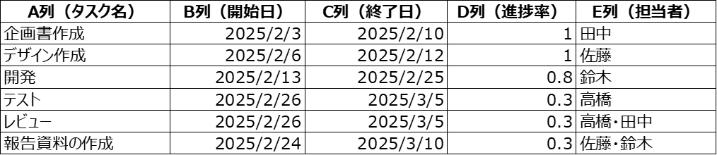
入力用シート(「タスク入力」)
タスク名・開始日・終了日・進捗率・担当者を入力しておくシートです。
出力用シート(「ガントチャート」)
マクロを実行すると、こちらのシート上にガントチャートが作成されます。
全体の処理の流れ
既存のガントチャートシートをクリア
タスクの最終行や日付の最小値・最大値を取得
日付のヘッダー(年月、日)を作成
タスクごとにガントバー(期間の色塗り)を表示
進捗率に応じて色を分ける
罫線や列幅の調整、ウィンドウ枠の固定
このように、「タスク入力」シートの情報をもとにして、自動でガントチャートの見た目まで整えてくれるのが大きな特徴です。
2. コードの説明
以下が今回紹介するVBAコードです。ExcelのVBAエディタに貼り付けて使います。
Sub CreateGanttChart()

    Dim wb As Workbook
    Dim wsInput As Worksheet, wsChart As Worksheet
    Set wb = ThisWorkbook
    Set wsInput = wb.Sheets("タスク入力")
    Set wsChart = wb.Sheets("ガントチャート")

    '――――――――――――――――――――――――――――――
    ' 既存のガントチャートシートをクリア
    '――――――――――――――――――――――――――――――
    wsChart.Cells.Clear

    '――――――――――――――――――――――――――――――
    ' タスクデータの最終行を取得(タスク入力は2行目以降)
    '――――――――――――――――――――――――――――――
    Dim lastRow As Long, i As Long
    lastRow = wsInput.Cells(wsInput.Rows.Count, "A").End(xlUp).Row
    If lastRow < 2 Then
        MsgBox "タスクデータが入力されていません。", vbExclamation
        Exit Sub
    End If

    '――――――――――――――――――――――――――――――
    ' タスクに含まれる日付範囲を求める(入力チェック付き)
    '――――――――――――――――――――――――――――――
    Dim minDate As Date, maxDate As Date
    Dim taskStart As Date, taskEnd As Date
    Dim firstTaskFound As Boolean
    firstTaskFound = False
    For i = 2 To lastRow
        If wsInput.Cells(i, 1).Value <> "" Then
            ' 入力チェック:開始日または終了日が入力されていない場合
            If Not IsDate(wsInput.Cells(i, 2).Value) Or Not IsDate(wsInput.Cells(i, 3).Value) Then
                MsgBox "タスク「" & wsInput.Cells(i, 1).Value & "」の開始日または終了日が入力されていません。", vbExclamation
                Exit Sub
            End If

            taskStart = CDate(wsInput.Cells(i, 2).Value)
            taskEnd = CDate(wsInput.Cells(i, 3).Value)
            ' 入力チェック:終了日が開始日より早い場合
            If taskEnd < taskStart Then
                MsgBox "タスク「" & wsInput.Cells(i, 1).Value & "」の終了日は開始日より早いです。", vbExclamation
                Exit Sub
            End If

            If Not firstTaskFound Then
                minDate = taskStart
                maxDate = taskEnd
                firstTaskFound = True
            Else
                If taskStart < minDate Then minDate = taskStart
                If taskEnd > maxDate Then maxDate = taskEnd
            End If
        End If
    Next i
    If Not firstTaskFound Then
        MsgBox "有効なタスクデータが見つかりません。", vbExclamation
        Exit Sub
    End If

    '――――――――――――――――――――――――――――――
    ' 表示範囲に余裕を持たせる(前後に1日追加)
    '――――――――――――――――――――――――――――――
    minDate = minDate - 1
    maxDate = maxDate + 1
    Dim totalDays As Long
    totalDays = maxDate - minDate + 1

    '────────────────────────────
    ' ヘッダー部設定(A~C列は1行目と2行目を結合)
    '────────────────────────────
    With wsChart.Range("A1:A2")
        .Merge
        .Value = "タスク名"
        .HorizontalAlignment = xlCenter
        .VerticalAlignment = xlCenter
        .Font.Bold = True
    End With
    With wsChart.Range("B1:B2")
        .Merge
        .Value = "担当者"
        .HorizontalAlignment = xlCenter
        .VerticalAlignment = xlCenter
        .Font.Bold = True
    End With
    With wsChart.Range("C1:C2")
        .Merge
        .Value = "進捗率"
        .HorizontalAlignment = xlCenter
        .VerticalAlignment = xlCenter
        .Font.Bold = True
    End With

    ' タイムラインは D列以降に表示
    Dim colStart As Long
    colStart = 4   ' タイムライン開始列

    Dim currentDate As Date
    Dim dayCounter As Long
    ' 2行目:各日の「日」数字、1行目:一旦日付をセット(後で月ごとにマージ)
    For dayCounter = 0 To totalDays - 1
        currentDate = minDate + dayCounter
        With wsChart.Cells(2, colStart + dayCounter)
            .Value = Day(currentDate)
            .HorizontalAlignment = xlCenter
            .VerticalAlignment = xlCenter
        End With
        ' 一旦日付をセット(後で月ごとのマージに利用)
        wsChart.Cells(1, colStart + dayCounter).Value = currentDate
    Next dayCounter

    '────────────────────────────
    ' 1行目:月ごとにセルをマージして「YYYY/M」と表示
    '────────────────────────────
    Dim startColOfMonth As Long, currentMonth As Integer, currentYear As Integer
    startColOfMonth = colStart
    currentMonth = Month(minDate)
    currentYear = Year(minDate)

    Application.DisplayAlerts = False
    For dayCounter = 0 To totalDays
        If dayCounter = totalDays Or Month(minDate + dayCounter) <> currentMonth Then
            Dim mergeStart As Long, mergeEnd As Long
            mergeStart = startColOfMonth
            mergeEnd = colStart + dayCounter - 1
            With wsChart.Range(wsChart.Cells(1, mergeStart), wsChart.Cells(1, mergeEnd))
                .Merge
                .Value = currentYear & "/" & currentMonth   ' 例:2025/2
                .HorizontalAlignment = xlCenter
                .VerticalAlignment = xlCenter
                .Interior.Color = RGB(220, 230, 241)
                .Font.Bold = True
            End With
            If dayCounter < totalDays Then
                startColOfMonth = colStart + dayCounter
                currentMonth = Month(minDate + dayCounter)
                currentYear = Year(minDate + dayCounter)
            End If
        End If
    Next dayCounter
    Application.DisplayAlerts = True

    '────────────────────────────
    ' 各タスクのガントバー作成
    '────────────────────────────
    ' タスク行は 3行目から
    Dim taskRow As Long
    taskRow = 3
    For i = 2 To lastRow
        If wsInput.Cells(i, 1).Value <> "" Then
            Dim tName As String, tStart As Date, tEnd As Date, tProgress As Double, tPerson As String
            tName = wsInput.Cells(i, 1).Value
            ' ここでは入力チェック済みのため、直接変換
            tStart = CDate(wsInput.Cells(i, 2).Value)
            tEnd = CDate(wsInput.Cells(i, 3).Value)
            tProgress = Val(wsInput.Cells(i, 4).Value)
            tPerson = wsInput.Cells(i, 5).Value

            ' タスク名(A列)、担当者(B列)、進捗率(C列)を表示
            With wsChart.Cells(taskRow, 1)
                .Value = tName
                .HorizontalAlignment = xlLeft
                .VerticalAlignment = xlCenter
            End With
            With wsChart.Cells(taskRow, 2)
                .Value = tPerson
                .HorizontalAlignment = xlCenter
                .VerticalAlignment = xlCenter
            End With
            With wsChart.Cells(taskRow, 3)
                .Value = tProgress
                .NumberFormat = "0%"  ' 進捗率を%表示
                .HorizontalAlignment = xlCenter
                .VerticalAlignment = xlCenter
            End With

            ' タイムライン上での位置を算出(D列以降)
            Dim startOffset As Long, endOffset As Long
            startOffset = tStart - minDate + 1   ' +1: 最初の日がタイムラインの1列目(D列)に対応
            endOffset = tEnd - minDate + 1

            ' ガントバー(タスク期間)の表示
            Dim barRange As Range
            Set barRange = wsChart.Range(wsChart.Cells(taskRow, colStart + startOffset - 1), _
                                         wsChart.Cells(taskRow, colStart + endOffset - 1))
            With barRange
                .Interior.Color = RGB(173, 216, 230)   ' ライトブルー
                .BorderAround LineStyle:=xlContinuous, Weight:=xlThin, Color:=RGB(0, 112, 192)
            End With

            ' 進捗率に応じたバー(左側から濃いブルーで塗りつぶす)
            Dim totalTaskDays As Long, progressDays As Long
            totalTaskDays = endOffset - startOffset + 1
            progressDays = Application.WorksheetFunction.Round(totalTaskDays * tProgress, 0)
            If progressDays > 0 Then
                Dim progressRange As Range
                Set progressRange = wsChart.Range(wsChart.Cells(taskRow, colStart + startOffset - 1), _
                                                  wsChart.Cells(taskRow, colStart + startOffset + progressDays - 2))
                progressRange.Interior.Color = RGB(0, 112, 192)   ' 濃いブルー
            End If

            taskRow = taskRow + 1
        End If
    Next i

    '────────────────────────────
    ' 列幅の調整
    '────────────────────────────
    wsChart.Columns(1).ColumnWidth = 20   ' タスク名
    wsChart.Columns(2).ColumnWidth = 15   ' 担当者
    wsChart.Columns(3).ColumnWidth = 10   ' 進捗率
    Dim j As Long
    For j = colStart To colStart + totalDays - 1
        wsChart.Columns(j).ColumnWidth = 3
    Next j

    ' 全体に外枠の罫線を引く
    wsChart.Range(wsChart.Cells(1, 1), wsChart.Cells(taskRow - 1, colStart + totalDays)).Borders.LineStyle = xlContinuous

    '────────────────────────────
    ' Freeze Panes:セル D3 を起点に固定(A~C列、1~2行固定)
    '────────────────────────────
    wsChart.Activate
    wsChart.Range("D3").Select
    ActiveWindow.FreezePanes = True

    wsChart.Cells(1, 1).Select
    MsgBox "ガントチャートの作成が完了しました。", vbInformation

End Sub
3. 使い方
Excelブックの準備
「タスク入力」シートと「ガントチャート」シートの2つを用意します。
「タスク入力」シートには、以下のような形でデータを入力します(行は2行目から)
何行でも追加できます
進捗率は0-1の間で入力します
VBAコードの貼り付け
VBAエディタ(Alt + F11)を開き、標準モジュールなどに今回のコードを貼り付けます。
マクロ実行
作成したマクロ(CreateGanttChart)を実行します。
成功すると、「ガントチャート」シートに自動で見やすい形のガントチャートが生成されます。
4. ファイルの配布
実際のファイルも置いておきます。これをダウンロードして使用することも可能です。
5. まとめ
Excelでガントチャートを手動で作るのは大変ですが、VBAを活用することで、タスク一覧を入力するだけで瞬時にガントチャートを生成できます。
今回ご紹介したコードは、比較的シンプルな構成になっているため、初心者の方でも改造や応用がしやすいはずです。「タスク入力」シートの項目を増やしたり、ガントバーの色や書式を変えてみたりといったカスタマイズをして、自分仕様のガントチャートを作ってみてください。
この記事で紹介したマクロをさらにカスタマイズしたい場合や、エラーが発生する場合は、お気軽にコメントをお寄せください!
※本記事で紹介しているマクロやファイルの使用に伴い発生したいかなるトラブルや損害についても、当方では一切の責任を負いかねます。すべて自己責任のもとでご利用ください。