kaggle:住宅価格の予測(Feature Engineering 1/3 (予定))

しばらく、データサイエンスの勉強から遠ざかっていたので、kaggleの人のnotebookを見ながら、写経&勉強。 備忘録を兼ねて、noteにしてみます。
データなどは、こちらから入手できます。
House Prices: Advanced Regression Techniques
参考にしたのは、こちらのnotebook
Comprehensive data exploration with Python
SalePriceの分布の確認
まずはデータを読み込んでみるんですが、とにかく沢山のデータが含まれています。
手始めに、一応価格予測をしたい以上、価格(SalePrice)がどのような分布をしているのかヒストグラムくらいは作ってみよう。
#invite people for the Kaggle party
import pandas as pd
import matplotlib.pyplot as plt
import seaborn as sns
import numpy as np
from scipy.stats import norm
from sklearn.preprocessing import StandardScaler
from scipy import stats
import warnings
warnings.filterwarnings('ignore')
%matplotlib inline

df_train = pd.read_csv('./input/train.csv')
#histgram
fig = plt.figure(figsize=(20,10))
ax1 = fig.add_subplot(1,2,1)
ax2 = fig.add_subplot(1,2,2)
ax1.hist(df_train['SalePrice'], bins=20)
ax2.hist(df_train['SalePrice'], bins=np.logspace(4,6,20))
ax2.set_xscale('log')
左はx軸(価格)が通常の(実数)表示
右はx軸(価格)が対数表示
最初、実数表示でヒストグラムを表示したら(予想通り)、左右対称ではない、右に裾が長い分布になっていた。対数表示(右)にしてみたら、左右対称に近く、正規分布っぽい形になった。
価格を学習させるときには対数化してからの方が良さそう。
参考にしたページ
データの精査
機械学習に読み込ませる特徴量(Feature )を、まずは理解しないと始まらないので、どのような特徴量(Feature )があるかを確認する。
df_train.columns

Index(['Id', 'MSSubClass', 'MSZoning', 'LotFrontage', 'LotArea', 'Street',
      'Alley', 'LotShape', 'LandContour', 'Utilities', 'LotConfig',
      'LandSlope', 'Neighborhood', 'Condition1', 'Condition2', 'BldgType',
      'HouseStyle', 'OverallQual', 'OverallCond', 'YearBuilt', 'YearRemodAdd',
      'RoofStyle', 'RoofMatl', 'Exterior1st', 'Exterior2nd', 'MasVnrType',
      'MasVnrArea', 'ExterQual', 'ExterCond', 'Foundation', 'BsmtQual',
      'BsmtCond', 'BsmtExposure', 'BsmtFinType1', 'BsmtFinSF1',
      'BsmtFinType2', 'BsmtFinSF2', 'BsmtUnfSF', 'TotalBsmtSF', 'Heating',
      'HeatingQC', 'CentralAir', 'Electrical', '1stFlrSF', '2ndFlrSF',
      'LowQualFinSF', 'GrLivArea', 'BsmtFullBath', 'BsmtHalfBath', 'FullBath',
      'HalfBath', 'BedroomAbvGr', 'KitchenAbvGr', 'KitchenQual',
      'TotRmsAbvGrd', 'Functional', 'Fireplaces', 'FireplaceQu', 'GarageType',
      'GarageYrBlt', 'GarageFinish', 'GarageCars', 'GarageArea', 'GarageQual',
      'GarageCond', 'PavedDrive', 'WoodDeckSF', 'OpenPorchSF',
      'EnclosedPorch', '3SsnPorch', 'ScreenPorch', 'PoolArea', 'PoolQC',
      'Fence', 'MiscFeature', 'MiscVal', 'MoSold', 'YrSold', 'SaleType',
      'SaleCondition', 'SalePrice'],
     dtype='object')
これらのデータがどういう意味なのかは、データと一緒についてくる data_description.txt というファイルに書いてある。
不動産の取引データなので、建物に関する情報だらけなのですが、米国の建物に関する用語が分からないので、地道に調べる。
MSSubClass: Identifies the type of dwelling involved in the sale.
どのような分類で売られていたかというカテゴリー変数。こんな感じ。
20 1-STORY 1946 & NEWER ALL STYLES
30 1-STORY 1945 & OLDER
40 1-STORY W/FINISHED ATTIC ALL AGES
45 1-1/2 STORY - UNFINISHED ALL AGES
他のデータで代用できるので、分析に含める必要はないかな。
MSZoning: Identifies the general zoning classification of the sale.
日本でも「住宅地域」「工業地域」という分類があるが、それと同じようなものか

RL Residential Low Density
RM Residential Medium Density
FV Floating Village Residential (水の上に浮いているような住居)
RH Residential High Density
C Commercial
一応、カテゴリー変数として分析に使えそう。
LotFrontage: Linear feet of street connected to property
(2020/9/19修正) 道路から建物までの直線距離、、、ではなく、土地の「間口」の長さ。土地が道路と接しているとき、その一辺の長さ。角地など2辺が道路と接しているような場合でも、代表的な一辺の長さを表している模様。 欠損値が259ある。

df_train['LotFrontage'].isnull().sum()

> 259
LotArea: Lot size in square feet
土地の広さ。これは、確実に住宅価格に影響するでしょう。
これも describe() で概要を見ると、土地の広い方に異常値があるようで、
50000スクエアフィート(4645平米)以上の広さの物件が11件、
100000スクエアフィート(9290平米)以上の広さの物件が4件あった。
これも対数に変換した方が、扱いやすい感じ。

fig = plt.figure(figsize=(20,10))
ax1 = fig.add_subplot(1,2,1)
ax2 = fig.add_subplot(1,2,2)

ax1.hist(df_train['LotArea'], bins=40)
ax2.hist(df_train['LotArea'], bins=np.logspace(3,6,40))
ax2.set_xscale('log')

Street: Type of road access to property
Grvl Gravel 砂利道
Pave Paved
自宅までの道路がが砂利道か舗装された道か、というパラメータだけど、1460件あるデータのなかで、砂利道というのは6件のみ。
無視しても影響はなさそうな、そんな感じ。売買がなされた年が 2006-2010年なので、そりゃほとんど舗装されてるでしょう。
df_train['YrSold'].describe()

> count    1460.000000
> mean     2007.815753
> std         1.328095
> min      2006.000000
> 25%      2007.000000
> 50%      2008.000000
> 75%      2009.000000
> max      2010.000000
Alley: Type of alley access to property
Grvl Gravel
Pave Paved
NA No alley access
自宅に至るalley(小道)が舗装されているか。road / alley がどう違うのか、ちょっとよく分からない。と思ったら、ほとんどが入力されていない欠損値。
無視してもよさそう。
df_train['Alley'].isnull().sum()
> 1369
LotShape: General shape of property
Reg Regular # 多分、綺麗な長方形なんだろう
IR1 Slightly irregular # 台形?
IR2 Moderately Irregular
IR3 Irregular # ???
土地の形状。四角いかとか、そういうことらしい。
一応、カテゴリー変数として扱ってみても良いのかもしれないが、IR2 / IR3 は数が少ないので、一つのカテゴリーにしても良いかも。
df_train['LotShape'].value_counts()

>Reg    925
>IR1    484
>IR2     41
>IR3     10
Name: LotShape, dtype: int64
LandContour: Flatness of the property
Lvl Near Flat/Level 平坦
Bnk Banked - Quick and significant rise from street grade to building
道路から建物まで上り坂
HLS Hillside - Significant slope from side to side
Bnk と HLS が用意されているところを見ると、道路からみて左右に斜めになっている、ということか。
Low Depression 窪地
df_train['LandContour'].value_counts()

> Lvl    1311> Bnk      63
> HLS      50
> Low      36
> Name: LandContour, dtype: int64
Utilities: Type of utilities available
いわゆるインフラがどれだけ整備されているか。
AllPub : All public Utilities (E,G,W,& S) Electricity, Gas, Water an Sewage
(下水道)
NoSewr : Electricity, Gas, and Water (Septic Tank) (汚水浄化槽)
NoSeWa : Electricity and Gas Only
ELO : Electricity only
sewage とか septic tank とか、英語の勉強にはなったけれど、1件を除き、全てインフラ整備されているようなので、機械学習には不要かな。
df_train['Utilities'].value_counts()

> AllPub    1459
> NoSeWa       1
> Name: Utilities, dtype: int64
LotConfig: Lot configuration
土地の仕様? google先生に画像を探してもらった。
なんとなく分かった気にはなったが、 FR2 / FR3 の違いはなんだかよく分からない。
Inside Inside lot
Corner Corner lot
CulDSac Cul-de-sac (袋小路)
FR2 Frontage on 2 sides of property
FR3 Frontage on 3 sides of property

出典:https://www.planning.org/pas/reports/report165.htm

cul de sac (袋小路) の例
出典:https://urbanprojectization.com/2019/06/29/what-is-a-cul-de-sacs/
df_train['LotConfig'].value_counts()
> Inside     1052
> Corner      263
> CulDSac      94
> FR2          47
> FR3           4
> Name: LotConfig, dtype: int64
一応、カテゴリー変数として扱ってみた方が良さそう。なんとなくのイメージだけど、Cul de sac って、高級住宅街にありそうな感じ。 FR2 / FR3 は、一つのカテゴリーで良さそう。
LandSlope: Slope of property
Slope という位だから、土地の傾斜?なんだかよく分からない。
上の "LandContour: Flatness of the property" と、どう違うのだろう。
Gtl Gentle slope
Mod Moderate Slope
Sev Severe Slope
df_train['LandSlope'].value_counts()

> Gtl    1382
> Mod      65
> Sev      13
> Name: LandSlope, dtype: int64
ほとんどが Gtl に分類されているので、無視してみる。
Neighborhood: Physical locations within Ames city limits
地域名のようだ。Ames city という都市のデータだということが分かる。
アイオワ州の中心部にある都市で、2010年の人口は6万人弱。関東だと千葉県東金市くらいの規模らしい。アイオワ州立大学というのがあるそうな。
df_train['Neighborhood'].value_counts()

> NAmes      225
> CollgCr    150
> OldTown    113
> Edwards    100
> Somerst     86
> 以下略
Names : North Ames
CollgCr : College Creek
OldTown : Old Town
Edwards : Edwards
Somerst : Somerset
地域によって、価格差がありそうなので、これはカテゴリー変数として扱うのが良さそう。
Condition1 / Condition 2: Proximity to various conditions
幹線道路に近い、線路に近い、公園や緑地に近いといった情報
df_train['Condition1'].value_counts()

> Norm      1260
> Feedr       81
> Artery      48
> RRAn        26
> PosN        19
> RRAe        11
> PosA         8
> RRNn         5
> RRNe         2
> Name: Condition1, dtype: int64

df_train['Condition2'].value_counts()

> Norm      1445
> Feedr        6
> RRNn         2
> PosN         2
> Artery       2
> RRAn         1
> PosA         1
> RRAe         1
> Name: Condition2, dtype: int64
ただ、大部分が Norm (Normal) というデータ。
公園や緑地に近いというプラス要素を示す PosN, PosA はほとんどない。
Feedr は、支線道路(feeder street) に近いという意味だそうだが、Normの7%くらいしかないので、無視しておこう。
BldgType: Type of dwelling 住居のタイプ
df_train['BldgType'].value_counts()

> 1Fam      1220
> TwnhsE     114
> Duplex      52
> Twnhs       43
> 2fmCon      31
> Name: BldgType, dtype: int64
1Fam : Single-family Detached
2FmCon : Two-family Conversion; originally built as one-family dwelling
Duplx : Duplex
TwnhsE : Townhouse End Unit
TwnhsI : Townhouse Inside Unit
1Fam は、普通の1世帯用の家だというのは分かる。アイオワの1世帯というのが何人くらいのイメージなのかは分からないけど。
Townhouse End Unit / Townhouse Inside Unit とはなじみがないので調べてみた。
https://www.bankrate.com/real-estate/what-is-a-townhouse/に説明と、下の写真があった。一応、全ての家の室内空間は独立しているが、隣の家と壁を共有している、、、というのが Townhouse の定義だそうな。独立した1戸建てよりも安く、お求めやすいようです。

機械学習にかける、という意味では 1Fam or NOT という区分で良さそう。
HouseStyle: Style of dwelling
住居のスタイル?
df_train['HouseStyle'].value_counts()

> 1Story    726
> 2Story    445
> 1.5Fin    154
> SLvl       65
> SFoyer     37
> 1.5Unf     14
> 2.5Unf     11
> 2.5Fin      8
> Name: HouseStyle, dtype: int64
1Story : 1階建て 2Story : 2階建て は分かる。
1.5Fin : One and one-half story: 2nd level finished
1.5Unf : One and one-half story: 2nd level unfinished
2階部分が finished / unfinished って、どういうこと? 完成してないの?
まあ、後で出てくる「地上階の総床面積」で代替が効くと思われるので無視しよう。
OverallQual: Rates the overall material and finish of the house
OverallCond: Rates the overall condition of the house
10 : Very Excellent から 1 Very Poor までの値を取る、、というが、相関関係ありそう。クロス集計表を出してみると、こんな感じ。
想像するに、、、
黄色の部分がボリュームゾーン、
黄色を除いた赤の部分が、ちょっと高くても良さそうな部分、
それ以外の部分はちょっと安そうな部分、、、となりそう。
3つのカテゴリーに分類して、機械学習にかけてみよう。

YearBuilt: Original construction date
YearRemodAdd: Remodel date (same as construction date if no remodeling or additions)
建築年と改築年
左のグラフが建築年 右のグラフが改築年
改築年のデータは 1950年以前のものが無いようなので、建築年のデータだけ使ってみよう。

RoofStyle: Type of roof
Flat : Flat
Gable : Gable 切り妻、破風 (赤毛のアン)
Gambrel : Gabrel (Barn)
Hip : Hip
Mansard : Mansard
Shed : Shed 斜面になった屋根

Gable は、"Anne of Green Gables" (赤毛のアン)のタイトルで聞いたことがあるけど、こういうタイプの三角屋根のことなんですね。屋根の形が住宅価格に影響するとも思えないので、無視しよう。

しばらく、価格に影響しなさそうなデータが続くので、端折っていこう。
ここから、外壁等の素材~
RoofMatl: Roof material (屋根の材質)
Exterior1st: Exterior covering on house
Exterior2nd: Exterior covering on house (if more than one material)
外壁の素材
MasVnrType: Masonry veneer type (レンガ壁の積み方)
MasVnrArea: Masonry veneer area in square feet (レンガ壁の広さ)
ExterQual: Evaluates the quality of the material on the exterior
ExterCond: Evaluates the present condition of the material on the exterior
外壁などのQualtiy / Condition (Overall Quality / Condition の内数?)
Foundation: Type of foundation (基礎)
ここから、地下室関係~
BsmtQual: Evaluates the height of the basement (地下室の天井の高さ)
BsmtCond: Evaluates the general condition of the basement (地下室の状態)
BsmtExposure: Refers to walkout or garden level walls
BsmtFinType1: Rating of basement finished area (地下室が居住可能か?)
BsmtFinType2: Rating of basement finished area (if multiple types)
BsmtFinSF1: Type 1 finished square feet
BsmtFinSF2: Type 2 finished square feet
BsmtUnfSF: Unfinished square feet of basement area
地下室の延べ床面積くらいは、データに入れてみよう。
TotalBsmtSF: Total square feet of basement area
Heating: Type of heating
大部分が GasA : Gas forced warm air furnace ガスで空気を暖めて、家全体を暖めるタイプのようです。 変数に使う必要はないかな。

HeatingQC: Heating quality and condition
Ex : Excellent Gd : Good TA: Typical & Average Fa:Fair Po:Poor
冬は寒そうなので、一応、カテゴリ変数として用いよう。

CentralAir: Central air conditioning
米国なので、ほとんどが Central heating だろうと思ったけど、その通り。
機械学習にかけるまでもなさそう。

Electrical: Electrical system
ブレーカーなのかヒューズなのか、というデータ。
ブレーカーの方が良いけれど、住宅価格に影響するとは思えない。
1stFlrSF: First Floor square feet
2ndFlrSF: Second floor square feet
LowQualFinSF: Low quality finished square feet (all floors)
GrLivArea: Above grade (ground) living area square feet
床面積関係の数値が四種類。居住用の地上の床面積を示す GrLivArea だけ採用。LotArea と同様、対数に変換した方が機械学習には良さそう。
fig = plt.figure(figsize=(20,10))
ax1 = fig.add_subplot(1,2,1)
ax2 = fig.add_subplot(1,2,2)

ax1.hist(df_train['GrLivArea'], bins=40)
ax2.hist(df_train['GrLivArea'], bins=np.logspace(2,4,40))
ax2.set_xscale('log')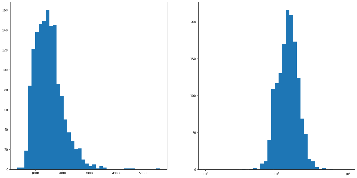
BsmtFullBath: Basement full bathrooms
BsmtHalfBath: Basement half bathrooms
FullBath: Full bathrooms above grade
HalfBath: Half baths above grade
バスルーム、トイレの数が住宅価格に影響するかなあ。。。 却下。
長くなったので、今日はここまで。。。