機械学習　混合行列

2023年10月9日 23:25

　クラス分類の機械学習アルゴリズムの性能を明らかにする混合行列を詳しく見ていく。

import pandas as pd
import matplotlib.pyplot as plt
import numpy as np

sklearnのデータセットから、ブレスト・キャンサーのデータセットをダウンロードし、これをデータフレームに入れる。

from sklearn.datasets import load_breast_cancer

cancer = load_breast_cancer()
df = pd.DataFrame(np.c_[cancer['data'], cancer['target']],
                  columns= np.append(cancer['feature_names'], ['target']))

df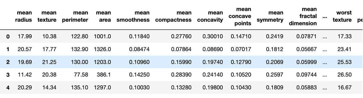

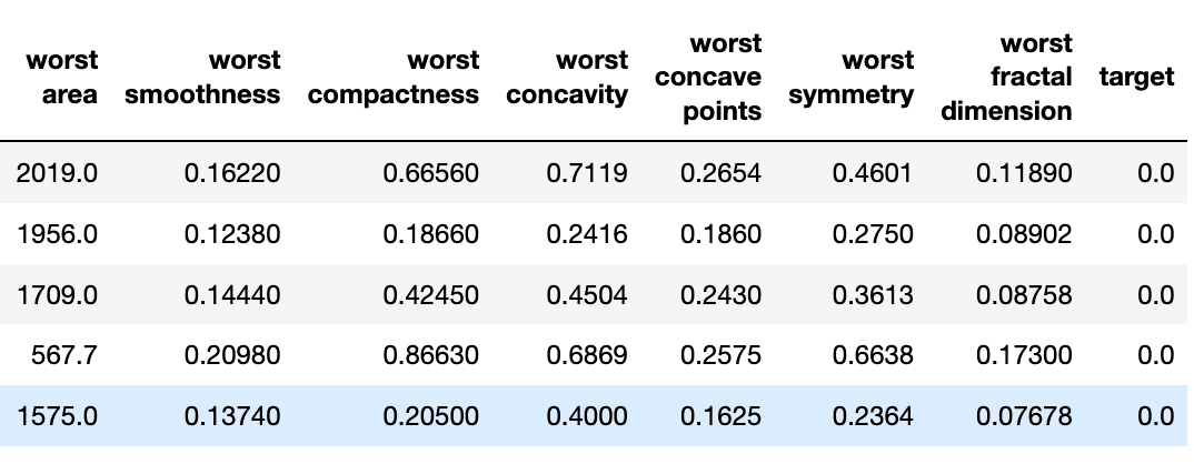
この最後の列が分類分けのターゲットとなるため、これを機械学習のyに、それ以前の列をxに入れ、訓練データとテストデータに分ける。

X = df.iloc[:,:-1].values
y = df.iloc[:, -1].values
from sklearn.model_selection import train_test_split

X_train, X_test, y_train, y_test = \
    train_test_split(X, y, 
                     test_size=0.20,
                     stratify=y,
                     random_state=1)

　訓練データをスケーリングし、サポートベクトルマシンに訓練データを渡すパイプラインを作成し、このテストと予測データから混合行列を表示する。

from sklearn.metrics import confusion_matrix
from sklearn.preprocessing import StandardScaler
from sklearn.pipeline import make_pipeline
from sklearn.svm import SVC

pipe_svc = make_pipeline(StandardScaler(),
                         SVC(random_state=1))
pipe_svc.fit(X_train, y_train)
y_pred = pipe_svc.predict(X_test)

confmat = confusion_matrix(y_true=y_test, y_pred=y_pred)

fig, ax = plt.subplots(figsize=(2.5, 2.5))
ax.matshow(confmat, cmap=plt.cm.Blues, alpha=0.3)
for i in range(confmat.shape[0]):
    for j in range(confmat.shape[1]):
        ax.text(x=j, y=i, s=confmat[i, j], va='center', ha='center')

plt.xlabel('Predicted label')
plt.ylabel('True label')

plt.tight_layout()
plt.show()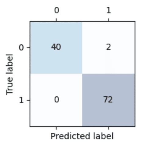

真陽性（TP:True Positive）True label=0, Prediction label=0
真陰性（TN:True Negative) True label=1, Prediction label=1
偽陽性（FP:False Positive）True label=1, Prediction label=0
偽陰性（FN:False Negative) True label=0, Prediction label=1

の分け方をする。
　これから、分類モデルの性能を示す以下の量が計算される。

誤分類率　$${ERR=\displaystyle{\frac{FP+TP}{TP+TN+FP+FN}}}$$
正解率　$${ACC=\displaystyle{\frac{TP+TN}{TP+TN+FP+FN}=1-ERR}}$$
偽陽性率　$${FPR=\displaystyle{\frac{FP}{TN+FP}}}$$
真陽性率　$${TPR=\displaystyle{\frac{TP}{TP+FN}}}$$
適合率　$${PRE=\displaystyle{\frac{TP}{TP+FP}}}$$
再現率　$${REC=\displaystyle{\frac{TP}{TP+FN}}}$$

再現率は真陽性率と同じである。
再現率の最適化は、FPの値を大きくし、適合率を上げることは、FNをも大きくする。
　よって、この適合率と再現率を組み合わせてバランスを取った、F1スコアが使われる。
$${F1=\displaystyle{\frac{PRE\times REC}{\frac{PRE+REC}{2}}}}$$

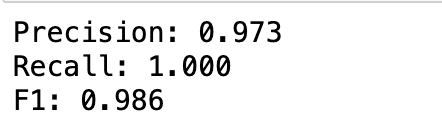
　これらの計算結果をsklearnから呼び出すのは次の通り。

from sklearn.metrics import precision_score, recall_score, f1_score

print('Precision: %.3f' % precision_score(y_true=y_test, y_pred=y_pred))
print('Recall: %.3f' % recall_score(y_true=y_test, y_pred=y_pred))
print('F1: %.3f' % f1_score(y_true=y_test, y_pred=y_pred))

機械学習 混合行列

いいなと思ったら応援しよう！

機械学習　混合行列