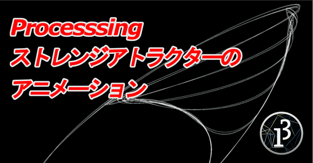
Processing でグラフを描く⑮ ストレンジアトラクターのアニメーション

Processing でグラフを描く 第15回目です。
前回「ストレンジアトラクター」に引き続き、この魅惑的な図形について調べていきます。前回の記事でストレンジアトラクターの発見と探索を行いました。簡単な式から変幻自在な図形が現れてくる様を観察することができました。
今回の課題は、ストレンジアトラクターの変化についてです。係数が少しずつ変化したとき、ストレンジアトラクターの形態はどう変わっていくのか。この変化を観察するにはアニメーションにするのが最適です。幸いにして Processing は簡単にアニメーションを作ることができます。
「ストレンジアトラクターのアニメーション」を作って遊んでみましょう。
ストレンジアトラクターの係数
$$
\begin{equation*}
\left\{ \,
\begin{aligned}
& x' =a_1 + a_2 x + a_3 x^2 + a_4 xy +a_5 y + a_6 y^2 \\
& y' =a_7 + a_8 x + a_9 x^2 + a_{10} xy +a_{11} y + a_{12} y^2 \\
\end{aligned}
\right.
\end{equation*}
$$
ストレンジアトラクターとは、上記の媒介変数 x, y によって表される x', y' を2次元平面上にプロットすることで作成できます。適切な係数 $${a_1, a_2, a_3…a_{12}}$$ を設定するときのみ、魅惑的な画像が得られます。
詳しい説明は、@KojiSaito様の「Sprott 式ストレンジアトラクタ発見機」に譲りますが、係数は「$${-1.2 <= a_n <=1.2}$$」までの値を 0.1 刻みで取ることがストレンジアトラクター作成上のルールとなっています。その25段階の数値をアルファベットの「A(-1.2) から Y(1.2)」に当てはめて、12文字からなる ID がストレンジアトラクターを表す名称(ID 識別番号)になっています。
ここで注意が必要なのは、係数の値を「$${-1.2 <= a_n <=1.2}$$ の範囲で 0.1 刻み」で限定したのは、一意の名称を与えるためであり、もっと細かい範囲でもストレンジアトラクターは作成できることです。
今回はその細かい範囲で係数を動かしたときの変化をアニメーションにします。そうすることで、係数とストレンジアトラクターの関係をより細かく観察することを目的としています。
アニメーション(ID: JGWMNTTGLLCD)
# strange attractor generator with Sprott's algorithm
# program by KojiSaito ( Twitter @KojiSaito )
# modified to animate by creativival
# import uuid

# If you set the ID, only one character will be different. If it is empty, a new one will be created.
# ID = ''
ID ='JGWMNTTGLLCD'
character_num = 0
InitX = InitY = .05
N = 10000
points_list = []


def init():
    global XE, YE, Lsum, Xmin, Xmax, Ymin, Ymax
    YE = .05
    XE = InitX + .000001
    Lsum = 0
    Xmin = Ymin = 1000000
    Xmax = Ymax = -Xmin
    id = [int(random(25)) for i in range(12)]
    coef = [(t - 12) * .1 for t in id]
    idStr = ""
    for c in id:
        idStr += chr(ord('A') + c)
    return coef, idStr


def next(coef, x, y):
    xNew = coef[0] + x * (coef[1] + coef[2] * x + coef[3] * y) + y * (coef[4] + coef[5] * y)
    yNew = coef[6] + x * (coef[7] + coef[8] * x + coef[9] * y) + y * (coef[10] + coef[11] * y)
    return xNew, yNew


def updateBound(x, y):
    global Xmin, Xmax, Ymin, Ymax
    Xmin = min(x, Xmin)
    Xmax = max(x, Xmax)
    Ymin = min(y, Ymin)
    Ymax = max(y, Ymax)


def LyapunovExponent(coef, x, y, n):
    global XE, YE, Lsum
    tx, ty = next(coef, XE, YE)
    dLx = tx - x
    dLy = ty - y
    dL2 = dLx * dLx + dLy * dLy
    df = 1e12 * dL2
    rs = 1 / sqrt(df)
    XE = x + rs * (tx - x)
    YE = y + rs * (ty - y)
    Lsum += log(df)
    return .721347 * Lsum / n  # L=Lyapunov exponent


def search(i):
    if ID == '':
        while True:
            coef, idStr = init()
            x, y = InitX, InitY
            found = True
            for i in range(1, 11000):
                x, y = next(coef, x, y)
                updateBound(x, y)
                l = LyapunovExponent(coef, x, y, i)
                if abs(x) + abs(y) > 1e6 or (i > 1000 and l < .002):  # Sprott 's original is .005
                    found = False
                    break
            if found:
                break
        print('ID="' + idStr + '"', " L=", l)
        return coef, idStr
    else:
        coef = [(ord(id) - 77) * .1 for id in ID]
        coef[character_num] = coef[character_num] - 0.1 + 0.001 * i
        print('ID="' + ID)
        return coef, ID


def calcScale(coef, w, h):
    init()
    x, y = InitX, InitY
    for i in range(1000):
        x, y = next(coef, x, y)
        updateBound(x, y)
    dx = .1 * (Xmax - Xmin)
    dy = .1 * (Ymax - Ymin)
    xl = Xmin - dx
    xh = Xmax + dx
    yl = Ymin - dy
    yh = Ymax + dy
    sx = w / (xh - xl)
    sy = h / (yh - yl)
    return sx, sy, xl, yl


def setColor(idStr):
    colorH = 538
    for c in idStr:
        colorH = ord(c) + colorH * 33
    colorH %= 251
    s = [0] * 3
    t = colorH % 3
    s[t] = 3
    s[(t + 1) % 3] = 1.5
    s[(t + 2) % 3] = .8
    colorMode(HSB, 250)
    c = color(colorH, 190, 200)  # make color here
    colorMode(RGB, 255)
    blendMode(ADD)
    plotColor = (s[0] * (red(c) + 40), s[1] * (green(c) + 40), s[2] * (blue(c) + 40))
    return plotColor


def drawSA(w, h, i):
    clear()
    Coef, IdStr = search(i)
    PlotColor = setColor(IdStr)
    sx, sy, tx, ty = calcScale(Coef, w, h)
    x, y = InitX, InitY
    points = [IdStr, PlotColor]
    for i in range(N):
        x, y = next(Coef, x, y)
        points.append(((x - tx) * sx, (y - ty) * sy))
    return points


def set_points():
    global points_list
    points_list = []
    for i in range(101):
        points_list.append(
            drawSA(width, height, i)
        )


def setup():
    size(1000, 1000)
    frameRate(1)
    set_points()


def draw():
    background(0)
    count = min(frameCount - 1, len(points_list) - 1)
    print(count)
    points = points_list[count]
    IdStr = points[0]
    PlotColor = points[1]
    stroke(PlotColor[0], PlotColor[1], PlotColor[2])
    for p in points[2:]:
        point(p[0], p[1])
    # information
    now_character = chr(ord(ID[character_num]) - 1)
    next_character = ID[character_num]
    text('ID: ' + IdStr, 5, 15)
    text('change position: ' + str(character_num), 5, 30)
    text('{} -> {} ({} %)'.format(now_character, next_character, str(count)), 5, 45)
    save_frame(0, 101)
上のアニメーションは、私が発見した ID: JGWMNTTGLLCD のストレンジアトラクターをアニメーションにしたものです。ポジション0 つまり先頭の係数 J(-0.3)に対して、I(-0.4) から 0.001 刻みで動かしたときのストレンジアトラクターの変化を記録したものです。
ストレンジアトラクターが膜状から線状に変化していく過程が捉えられています。1枚目から面白いのが出てきましたね。ワクワク。
# character_num = 0
character_num = 3
上のアニメーションは、ポジション3 つまり4番目の係数 M(-0.0)に対して、L(-0.1) から 0.001 刻みで動かしたときのストレンジアトラクターの変化を記録したものです。変化の大きいポジションをアニメーションの区間に選びました。
4つの点から薄い線が伸びてきて、急にストレンジアトラクターに変化します。面白いですね。この4つの始点がストレンジアトラクターの謎を解く鍵になるかもしれません(適当な感想です)。
# character_num = 0
# character_num = 3
character_num = 10
次は、ポジション10 つまり11番目の係数 C(-1.0)に対して、B(-1.1) から 0.001 刻みで動かしたときのストレンジアトラクターの変化を記録したものです。
4本の短い線が一度薄くなりますが、その後ストレンジアトラクターに急速に成長します。この変化は、分割したストレンジアトラクター(一つ以上のパーツを持つ)は、ある条件下で1つにまとまる可能性があるということかもしれません。
アニメーション(ID: SYHLDECORFNV)
ID ='SYHLDECORFNV'
character_num = 0
別のストレンジアトラクターで検証を続けます。 ID: SYHLDECORFNV のストレンジアトラクターをアニメーションにしたものです。ポジション0 つまり先頭の係数 S(0.4)に対して、R(0.5) から 0.001 刻みで動かしたときのストレンジアトラクターの変化を記録したものです。
膜状のストレンジアトラクターが形状を変えていきます。まるでアメーバーのようです。とがった角が伸びていくところが興味深いです。本当に生き物のようです。
# character_num = 0
character_num = 3
次は、ポジション3 つまり4番目の係数 L(-0.1)に対して、K(-0.2) から 0.001 刻みで動かしたときのストレンジアトラクターの変化を記録したものです。
こちらのアニメーションは変化が急激すぎて判別が難しいです。変化率 60% 前後をもっと細かく観察する必要がありそうです。
# character_num = 0
# character_num = 3
character_num = 8
最後に、ポジション8 つまり9番目の係数 R(0.5)に対して、O(0.4) から 0.001 刻みで動かしたときのストレンジアトラクターの変化を記録したものです。
この画像は、線状から膜状に変化する様子が捉えられています。ストレンジアトラクターの本質は膜状の形態ではなく、線状に収束した状態であることを示唆しているかもしれません。
ストレンジアトラクターの分類について
@KojiSaito 様より、ストレンジアトラクターの分類について意見を求められました。私はストレンジアトラクターで遊んでいるだけですから、単なる感想しか持っていませんが、今回のアニメーションから得たインスピレーションを書いてみます。
ストレンジアトラクターは、点、線、面(膜状)に収束するので、大分類はその3つにする。点は線に、面は線に収束する可能性があり、ストレンジアトラクター探索機で、周辺IDを調査し、線に収束するときは、そちらを採用する。(線状を基本形とする)
あとは、点の数(始点がわかれば、その数)、線の数、線の開く閉じる、面の数、突起の数あたりで分類してみると、ある程度のカタログができるのではないでしょうか? 読者の皆様のご意見も伺いたいですね。コメント欄で分類のアイデアがあれば教えてください。
一緒に #StrAttrCat を盛り上げていきましょう!
前の記事
Processing でグラフを描く⑭ ストレンジアトラクター
次の記事
Processing でグラフを描く⑯ ハーモノグラフ
その他のタイトルはこちら